Credit Risk Modelling: the Probability of Default

We will focus here on the probability of default, one of the key measure of credit risk, introducing different ways to measure it.

What is the Probability of Default?

The probability of default is the likelihood that a borrower, which can be an individual, a corporate or a government fails to meet its debt obligations within a specified time period. 

It is a crucial measure for lenders, investors, and financial institutions to assess and manage credit risk.

We will focus here on the probability of default for corporates and governments.

Factors Influencing the Probability of Default

There are different factors influencing the probability of default of a borrower, such as:

• Credit History: past behavior in debt repayment.
• Financial Health: income, expenses, debt, leverage, financial stability.
• Economic Conditions: economic downturns can increase default rates.
• Industry, Regional Risks: certain industries or regions can be more affected by an economic downturn.

How to Assess the Probability of Default?

There are different ways to assess the probability of default of a company or a government:

• Credit Rating: given by rating agencies like S&P, Moody’s, Fitch or internal
• Credit Score: numerical representation of the creditworthiness
• Statistical and Machine Learning Models: logistic regression, machine learning models
• Market Implied Default Probability: From market data using a default model

Credit Rating

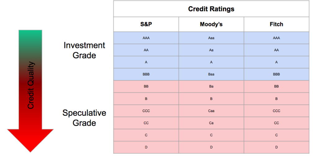
Standard & Poor’s, Moody’s and Fitch are the three major credit rating agencies, all three are American. They mainly rate corporate, financial institutions and countries.

Ratings are from AAA which is the highest rating to D which corresponds to default.

They have a significant impact, influencing borrowing costs and investment decisions.

Investment grades correspond to the highest ratings with the lowest probability of default, while speculative grades are the lowest rating with the highest risk of default.

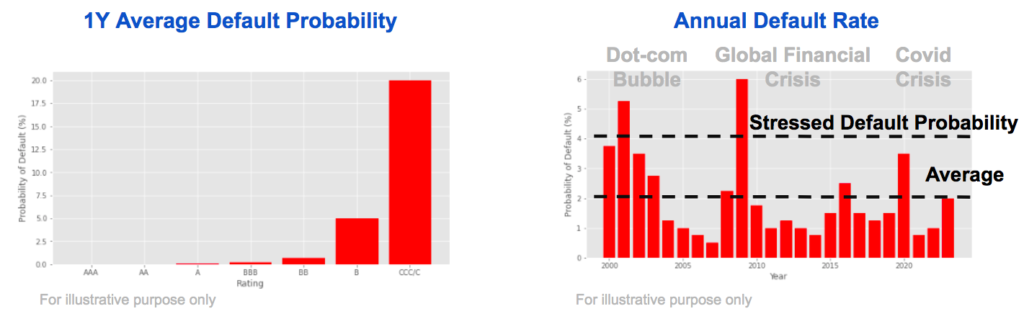
Rating agencies publish statistics on their data including the average default rate through the cycle.

We see that the default probability increases significantly when the credit quality deteriorates.

The default rate varies, with higher default rate during crisis periods,  allowing to asset default probability over different phases of the economic cycle.

Numbers here are purely illustrative.

Credit Score and Altman Z-Score

The credit score is a numerical representation of the creditworthiness.

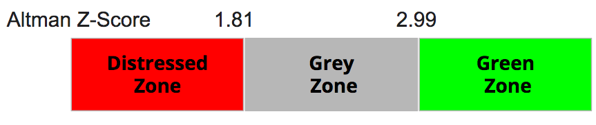
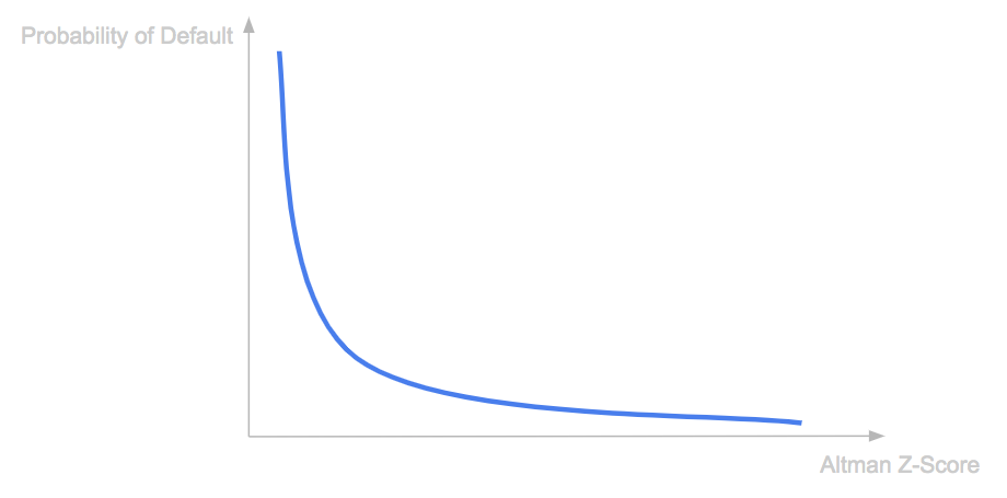
The Altman Z-Score is a famous scoring formula for predicting bankruptcy of corporate, first published in 1968 by Edward I. Altman.

It is mostly accounting based. Here is the original z-score formula for manufacturing companies.

Z = 1.2X₁ + 1.4X₂ + 3.3X₃ + 0.6X₄ + 1.0X₅

The z-score of a company is a function of five ratios:

• X₁ = working capital / total assets
• X₂ = retained earnings / total assets
• X₃ = earnings before interest and taxes / total assets
• X₄ = market value of equity / total liabilities
• X₅ = sales / total assets

If the z-score is below 1.81 the company is in distressed zone, with a higher risk of failure, while if the z-score is above 2.99 the company is in green zone with a low risk of default. The Grey zone is in-between.

Statistical and Machine Learning Models

The Z-Score itself does not directly provide a default probability, empirical studies and historical data can help estimate a mapping from Z-Scores to default probabilities.

One approach is to use logistic regression on historical data of companies’ Z-Scores and their subsequent default rates to estimate the probability of default.

First we collect historical data of companies with their Z-Scores and whether they defaulted or not.

Then we fit a logistic regression model and we can estimate the default probability.

Logistic regression can be done as well using a series of financial data (X_i)_i=1…n to estimate the default probability.

Exploratory data analysis, variable selection methods can be used to choose the most relevant variables to be included in the regression.

Machine learning classification techniques can be tested as well such as Decision Tree, Random Forests, Gradient Boosting Machines, Support Vector Machines or Neural Network.

Default Models

In order to estimate default probabilities from market data we need a default model.

There are two main families of default models:

• Structural models: based on the firm’s assets and liabilities (e.g., Merton model).
• Reduced-form models: focus on the timing of default (e.g., Jarrow-Turnbull model).

Structural Models, the Merton Model

Structural models are accounting based, the total asset of a company is equal to the sum of its equity and its debt.

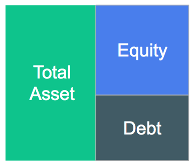
There is a default if the total asset of the company goes below its debt.

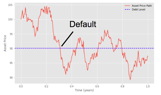
In the Merton Model, the company’s equity is modelled as a call option on its asset, we are in the Black-Scholes framework.

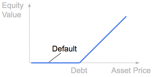
Without going much more into details in this article, in this framework the probability of default is a function of:

• The debt market value (D)
• The equity market value (E)
• The equity volatility (σ_E)
• The maturity of the debt (T)
• The risk-free interest rate (r)

PD = f(D, E, σ_E, T, r)

Reduced-Form Models

In reduced form models, defaults occur randomly, the default time is random and is driven by a default intensity process λ, we assume that lambda is deterministic here.

In this framework the default probability before T (PD_T) can be expressed as following, it is a function of the integral of λ_t between 0 and T.

It can be shown that if we assume a  constant default intensity λ we have the credit spread S which is very close to the product of lambda and 1 minus the recovery rate:

S ≈ λ x (1 – R)

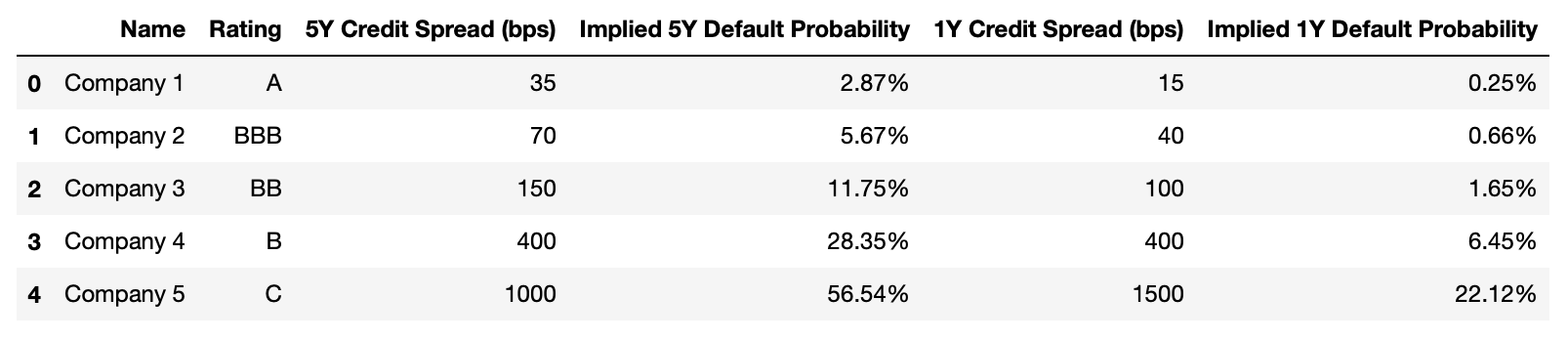
And so the default probability before T can be directly estimated from the credit spread if we fix the value of the recovery rate.

We fix the value of the recovery rate at 40% in the example below, which is the market convention for senior unsecured debts. For these five companies, we assume that we know the 5y credit spread. So we can estimate the five year default probability using the previous formula.

Similarly if we know the value of the 1Y credit spread we can estimate the 1Y default probability.

Watch the Video

Save 10% on All Quant Next Courses with the Coupon Code: QuantNextBlog10

For students and graduates: We offer a 50% discount on all courses, please contact us if you are interested: contact@quant-next.com