Pricing of a Defaultable Bond with a Reduced-Form Model (Part III, IV, V)

In the previous post (link) dedicated to the pricing of defaultable bonds with a reduced form model, we saw how to price a zero coupon bond and a bond paying coupons with zero recovery rate.

In this one we will see how to price a bond assuming a non zero recovery rate in case of default. We will discuss on the calibration of the model, on potential applications of the pricing model and we will compare different measures of credit spread.

III. Pricing of a Risky Bond with Recovery Rate

Pricing formula with no recovery rate in case of default

We consider a risky bond paying coupons. Coupons are paid as long as there is no default. Coupons are paid as long as there is no default. The principal amount is repaid at maturity in the absence of default. We assume zero recovery rate. In case of default, the bondholder will not recover any part of his initial investment.

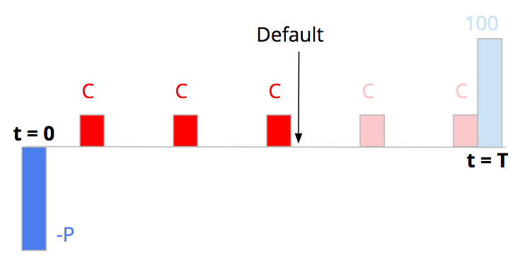
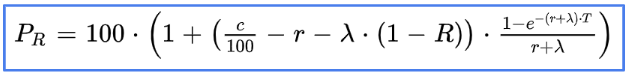
The price of the risky bond is the expectation of the sum of the discounted cash-flows, with continuous compounding it can be expressed as following (more details in the previous post):

Pricing of a risky bond with recovery rate

Now we assume as well that In case of default, the bondholder will recover a part of his initial investment.

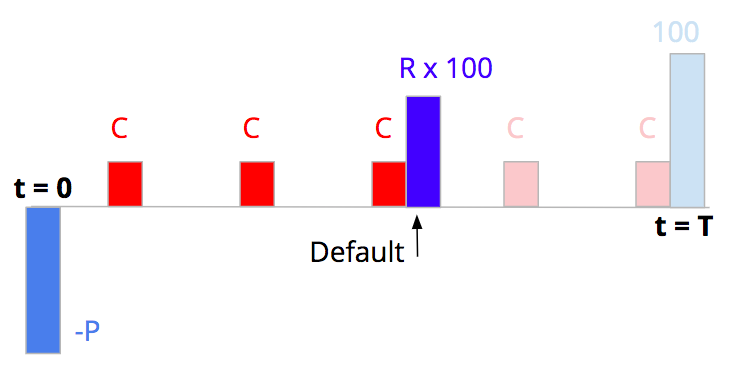
There is an additional cash-flow compared to the zero-recovery case, with the payment of the recovery rate R in case of default.

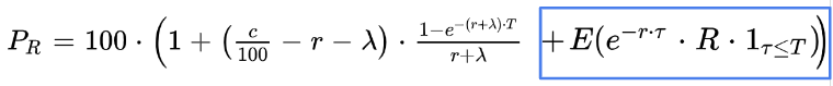
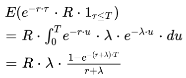
We assume that the time of default tau follows an exponential distribution:

and we obtain this expression for the expectation of the additional cash flow:

So the price of the risky bond can be written as following:

Credit spread

The previous expression makes appear the credit spread. The credit spread is the compensation for bearing a credit risk when purchasing the bond.

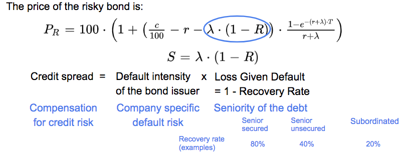
It is the product of the default intensity lambda and one minus the recovery rate R:

• The default intensity is a measure of the company’s default risk.
• One minus the recovery rate is the loss given default. It depends on the seniority of the debt. A senior secured debt will typically have a higher recovery rate compared to a senior unsecured debt. The subordinated debt will have lower priority in the repayment order in the event of default, with a lower recovery rate.

Probability of default and expected loss

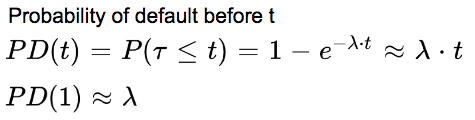
With a constant default intensity model, the probability of default is the cumulative distribution function of an exponential law. It is close to lambda time t with a first order taylor development. So lambda is close to the one year default probability.

With no discount rate, the expected loss before t is equal to the product of the default probability and 1 minus the recovery rate. So we see that the credit spread S, is close to the one year expected loss.

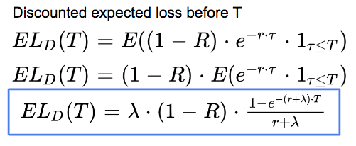
The discounted expected loss before T is equal to the product of the default probability before T and one mius the recovery rate only if the interest rate r is equal to 0.

If r is different from 0, we have to calculate the expectation of the discount factor between 0 and the default time tau. Using the probability density function of tau we obtain this expression for the discounted expected loss before T.

Going back to the price we recognize the discounted EL as the last term. The expected loss is the product of the credit spread, close to the one year expected loss and the risky duration, the duration of the bond taking into account the default risk.

Bond price decomposition

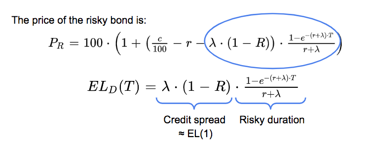
So the bond price is equal to 100 plus the difference between two terms.

• RPV(excess coupon): risky present value of the coupon in excess of the risk free interest rate.

• Expected Loss: the opposite of the discounted expected loss before T.

If the risky present value of the excess coupon is higher (resp. lower) than the discounted expected loss, the price of the bond will be above (resp. below) par. If the two are equal, the price of the bond will be at par, equal to 100.

IV. Credit spread vs z-spread

Bond price as a function of credit spread and z-spread

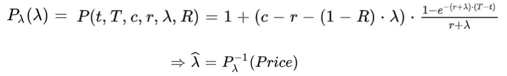
The default intensity λ can be expressed from the credit spreads S and the recovery rate R, so we can price the defaultable bond as a function of the credit spread:

The z-spread z is the spread that needs to be added to the risk free interest rate to obtain the price of the risky bond. It is the additional compensation asked by investor for taking that risk.
The price of the bond can be expressed as a function of the z-spread z assuming continuous compounding and constant interest rates:

When we compare two expressions of the bond price as a function of credit spread S and as a function of the z-spread z we immediately see that the two spreads are equal if and only if the recovery rate capital R is equal to zero.

Sensitivity of the z-spread to default intensity

We will know analyse the sensitivity of the z spread to the default intensity and to the coupon.

For that we need to be able to imply the z-spread from bond prices.

Here is a python code doing that. We minimise the square difference between the bond price P and the bond price as a function of the z=spread using the scipy optimize function minimize.

Python Code

import numpy as np
from scipy.optimize import minimize
import matplotlib.pyplot as plt
plt.style.use('ggplot')

# Bond price function with z spread
def BondPrice_zspread(t, T, c, r, z):
    return 100 * (1 + (c / 100 - r - z) \
                  * (1 - np.exp(-(r + z) * (T - t))) / (r + z))

#z-spread as a function of the bond price P
def Price_to_zspread(t, T, c, r, P):
    # Initial guess for z
    initial_guess = 0.01
    # Squared error (loss function to minimise)
    def loss(x):
        return (BondPrice_zspread(t, T, c, r, x) - P)**2 # Squared error
    # Use scipy.optimize.minimize to find the z-spread
    result = minimize(loss, x0=initial_guess)
    return result.x[0]

#parameters
t = 0
T = 10 # maturity in years
c = 4 # coupon
r = .03 # risk-free interest rate
P = 103 # bond price
z = Price_to_zspread(t, T, c, r, P)

print("z-spread:", np.round(z, 4))
print("Check bond price:", np.round(BondPrice_zspread(t, T, c, r, z),1))

For different values of the default intensity λ, all other parameters being fixed, we can price the bond (P_λ), and then calculate the corresponding z-spread.

We are doing that assuming a recovery rate at 0% and a recovery rate at 40%.

The z-spread z is equal to the default intensity lambda and to the credit spread S when the recovery rate is equal to zero.

When the recovery rate is not null, we see that the z-spread is below the credit spread S. This is to compensate for the additional cash flow as there is no assumption of recovery rate to calculate the z-spread. 

Parameters: T = 10yrs, r = 3%, R = 40%, c = 4

Python Code

# Bond price function with default intensity model
def BondPrice_intensity(t, T, c, r, R, lambda_):
    return 100 * (1 + (c / 100 - r - lambda_ * (1-R)) \
                  * (1 - np.exp(-(r + lambda_) * (T - t))) / (r + lambda_))

#parameters
t = 0
T = 10 # maturity in years
r = .03 # risk-free interest rate
R = .4 # recovery rate
c = 4 # coupon
Lambda = np.arange(0, .2, .001)
z_spreadR40 = []
for l in Lambda:
    P_ = BondPrice_intensity(t, T, c, r, R, l)
    z_ = Price_to_zspread(t, T, c, r, P_)
    z_spreadR40.append(z_)
z_spreadR0 = []
for l in Lambda:
    P_ = BondPrice_intensity(t, T, c, r, 0, l)
    z_ = Price_to_zspread(t, T, c, r, P_)
    z_spreadR0.append(z_)

plt.figure(figsize=(10, 6))
plt.plot(Lambda, z_spreadR40)
plt.plot(Lambda, z_spreadR0)
plt.plot(Lambda, Lambda * (1 - R))
plt.title('z-spread as a function of default intensity')
plt.xlabel('Default intensity')
plt.ylabel('z-spread')
plt.legend(['z-spread, Recovery rate = 40%', 'z-spread, \
Recovery rate = 0%', 'lambda x (1 - R)'])
plt.show();

Sensitivity of the z-spread to coupon

The credit spread S is the product of two variables. The default intensity which is issuer specific and 1 minus the recovery rate which is depending on the seniority of the bond. It is independent of the coupon of the bond.

λ: issuer specific, 1- R: depending on the seniority of the bond

So the credit spread is independent of the coupon of the bond.

This is not true for the z-spread which is depending on the coupon of the bond.

Here is a Python code calculating the z-spread of a bond for different values of the coupon. We see that the z-spread increases with the coupon of the bond.

It makes sense, as a higher coupon means a higher proportion of the coupon and a lower proportion of the recovery rate in case of default in the cash flows of the bond.

Python Code

#parameters
t = 0
T = 10 # maturity in years
r = .03 # risk-free interest rate
R = .4 # recovery rate
lambda_ = .01 # default intensity
Coupon = np.arange(1,20,1)
z_spread = []
for c in Coupon:
    P_ = BondPrice_intensity(t, T, c, r, R, lambda_)
    z_ = Price_to_zspread(t, T, c, r, P_)
    z_spread.append(z_)

plt.figure(figsize=(10, 6))
plt.plot(Coupon, z_spread)
plt.title('z-spread as a function of coupon')
plt.xlabel('Coupon')
plt.ylabel('z-spread')
plt.show();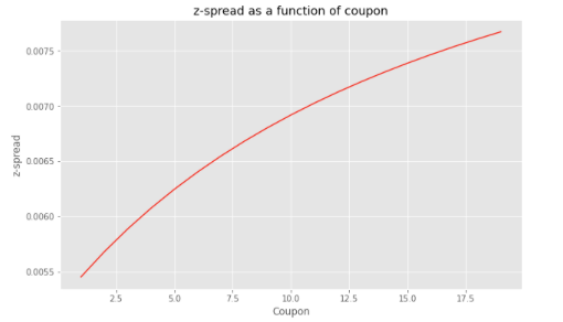

IV. Calibration of the parameters and applications

Calibration of the parameters

There are three parameters to be calibrated in our pricing model:

• Risk free rate r
• Recovery Rate R
• Default Intensity λ

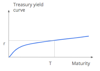
The risk free rate r can be estimated from Treasury bonds with similar tenor T.

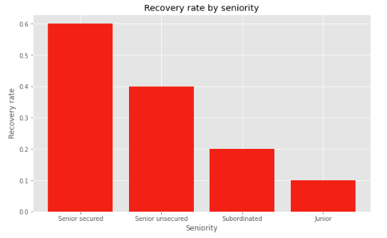
The recovery rate is depending on corporate bond seniority, the higher the seniority of the bond, the higher the expected recovery. 

Numbers here tend to be the market convention, in line with historical average recovery rates. The recovery rate of a senior unsecured bond would be typically 40%.

Knowing the recovery rate, the default intensity can be estimated from bonds of a similar issuer but with different maturities, seniorities and coupons by matching the bond prices.

In this illustration, we see that there is a term structure for the default intensity, which is a function of the tenor, with a higher default intensity for a higher tenor in this example.

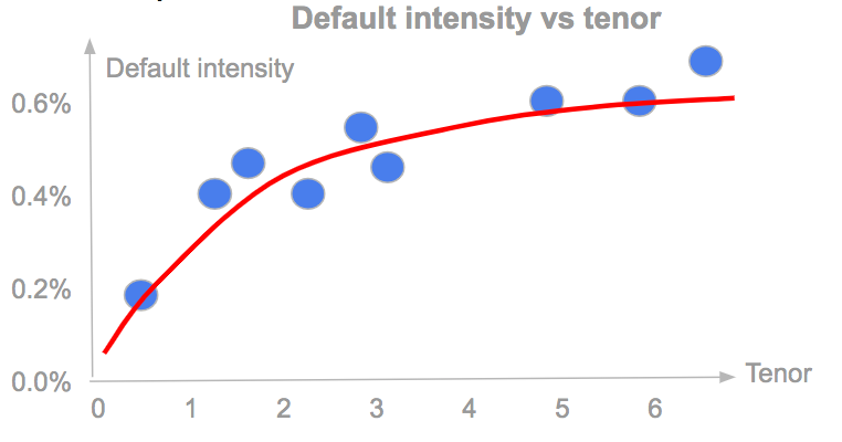
We can fit the curve with a parametric model, using for example a Nelson Siegel function which is popular in fixed income.

More advanced models, assuming non constant risk free interest rates and default intensity can be used to take into account the whole term structure of the curves in the pricing of the instrument.
Classical bootstrapping and interpolation methods to calibrate the discount factor (zero-coupon) curve from treasury curve.

The survival probability function can be estimated assuming a non-constant default intensity, deterministic time varying (piecewise constant or linear, with parametric functions) or stochastic (ex: Cox-Ingersoll-Ross process).

There are not always enough information from bonds on one single issuer, not enough bonds or tenors, to well calibrate the term structure.  

Additional informations from other bonds or other markets such as Credit Default Swap (CDS) may be required.

Applications

Here are several potential applications of the pricing model:

• Pricing of a new issuance
• Pricing of more complex bonds (hybrids, Cocos…) or products (derivatives, structured products)
• Relative value analysis:
  • Bond vs bond of a same issuer
  • Bond vs bond of different issuers
  • Bond vs CDS of a same company
• Risk management

Watch the Videos

Credit Risk Modelling: Pricing of a Defautable Bond with Reduced-Form Model Part III

Credit Risk Modelling: Pricing of a Defautable Bond with Reduced-Form Model Part IV

More about Credit Risk:

Credit Risk: an Introduction

Credit Risk Modelling: the Probability of Default

Credit Risk Modelling: the Default Time Distribution

An Introduction to Reduced-Form Credit Risk Models

Pricing of a Defaultable Bond with a Reduced-Form Model (Part I & II)

Save 25% on All Quant Next Courses with the Coupon Code: QuantNextBlog25

For students and graduates: We offer a 50% discount on all courses, please contact us if you are interested: contact@quant-next.com

List of Quant Next Courses

We summarize below quantitative finance training courses proposed by Quant Next. Courses are 100% digital, they are composed of many videos, quizzes, applications and tutorials in Python.

Complete training program:

Options, Pricing, and Risk Management Part I: introduction to derivatives, arbitrage free pricing, Black-Scholes model, option Greeks and risk management.

Options, Pricing, and Risk Management Part II: numerical methods for option pricing (Monte Carlo simulations, finite difference methods), replication and risk management of exotic options.

Options, Pricing, and Risk Management Part III:  modelling of the volatility surface,  parametric models with a focus on the SVI model, and stochastic volatility models with a focus on the Heston and the SABR models.

A la carte:

Monte Carlo Simulations for Option Pricing: introduction to Monte Carlo simulations, applications to price options, methods to accelerate computation speed (quasi-Monte Carlo, variance reduction, code optimisation).

Finite Difference Methods for Option Pricing: numerical solving of the Black-Scholes equation, focus on the three main methods: explicit, implicit and Crank-Nicolson.

Replication and Risk Management of Exotic Options: dynamic and static replication methods of exotic options with several concrete examples.

Volatility Surface Parameterization: the SVI Model: introduction on the modelling of the volatility surface implied by option prices, focus on the parametric methods, and particularly on the Stochastic Volatility Inspired (SVI) model and some of its extensions.

The SABR Model: deep dive on on the SABR (Stochastic Alpha Beta Rho) model, one popular stochastic volatility model developed to model the dynamic of the forward price and to price options.

The Heston Model for Option Pricing: deep dive on the Heston model, one of the most popular stochastic volatility model for the pricing of options.