Credit Risk Modelling: the Default Time Distribution

We will focus here on the default time distribution. We will see the relationship between the cumulative and the marginal default rates and how these two probabilities change with time depending on the credit quality of the borrower.

Default Event and Default Time

A default event refers to a situation where a borrower fails to meet its legal obligations of debt repayment. 

The default time (τ) is the point in time when the default event occurs, it is a random variable, following a certain distribution function.

Cumulative Default Probability and Survival Probability

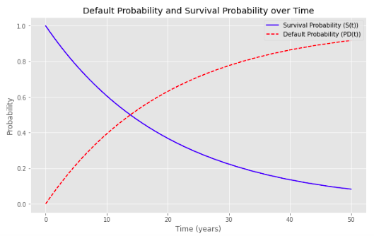
For a given borrower, the cumulative default probability PD(t) gives the probability of default between 0 and t.

The survival probability S(t) is the probability that there is no default before t.

The sum of the two is equal to 1.

The survival probability, in blue on this chart, starts at 100% and decreases over time converging to 0 while the default probability, in red, starts at 0 and increases over time converging to 1.

The default time density function (pdf) is the derivative of the cumulative default probability with respect to time. 

The probability that there is a default between t and t + dt is equal to pdf(t) x dt.

The integral between 0 and +∞ of pdf is equal to 1.

Default Time Distribution with Constant Default Intensity Model

A first simple example is the default time distribution with a constant default intensity model. 

The cumulative default probability is:

The survival probability is:

The default time density function is:

We recognize the probability density function of an exponential distribution with λ the parameter of the distribution.

λ is the hazard rate, also known as the default intensity or failure rate.

It represents the instantaneous rate at which a borrower is expected to default at any given time, given that he has not defaulted before:

On this chart, we show the default probability and the cumulative probability as a function of time with λ = 5%.

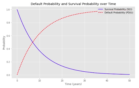
Default Probability and Survival Probability with λ = 5%

If λ increases, it means a higher risk of default for the borrower. The cumulative default probability function increases, converging more quickly to 1 while the survival probability decreases.

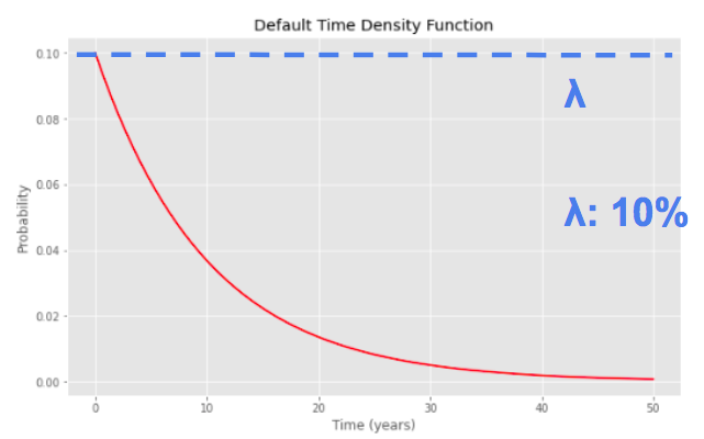
Default Probability and Survival Probability with λ = 10%

If we plot this time the default time density function still assuming a constant default intensity we see that it is a decreasing function of time, which makes sense as the survival probability decreases with time.

However, the conditional probability of default between t and t + dt in this framework remains constant equal to λ x dt.

Marginal Default Probability

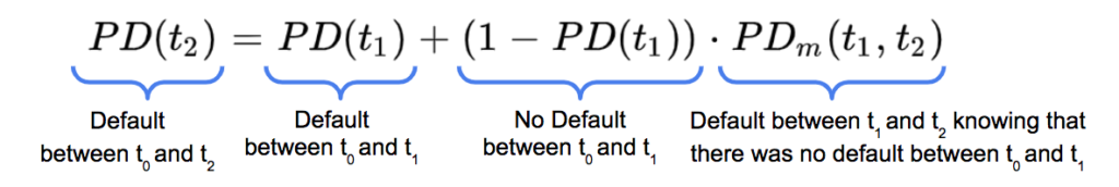
The marginal default probability is the probability that a borrower will default in a specific time period, given that it has survived up to the beginning of that period. 

If we know the cumulative default probability at t₁ and t₂ we can deduce the marginal default probability between t₁ and t₂ with the following expression.

Demo:

Cumulative and Marginal Default Rates as a Function of the Credit Quality

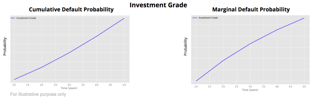
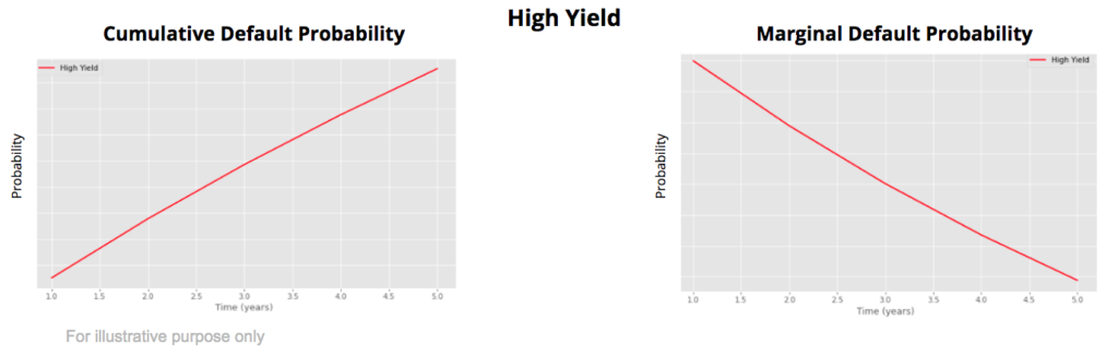
The evolution of the cumulative and marginal default probabilities depend on the credit quality of the borrower.

For an investment grade borrower with a good credit quality, the default risk is low on the short-term. However if the borrower does not default, there are risks that it will not able to maintain the same credit quality over time, that it downgrades over time meaning an increase of the marginal default probability.

For a high yield borrower with a bad credit quality it is the opposite. Its default probability is high on the short-term. But if it survives it is likely that it upgrades meaning a better credit quality over time and a decrease of the marginal default probability.

Exercise in Python

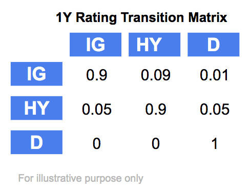
1/ Using this 1Y rating transition matrix, calculate the 2Y, 3Y, 4Y and 5Y cumulative transition matrices

2/ Plot the cumulative default rates for investment grade (IG) and high yield (HY) credit ratings

3/ Plot the corresponding marginal default rates

You will find the Python code at the end of the article.

Watch the Video

Save 10% on All Quant Next Courses with the Coupon Code: QuantNextBlog10

For students and graduates: We offer a 50% discount on all courses, please contact us if you are interested: contact@quant-next.com

Python Code

import numpy as np
x = np.array([[0.9,0.09,0.01], [0.05, 0.9, 0.05], [0, 0, 1]])
y = np.matrix(x)

PD_Cum_IG = []
PD_Cum_HY = []
PD_Marg_IG = []
PD_Marg_HY = []
for i in range(5):
    m = y**(i+1)
    PD_Cum_IG.append(m[0,2])
    PD_Cum_HY.append(m[1, 2])
    if (i == 0):
        PD_Marg_IG.append(PD_Cum_IG[0])
        PD_Marg_HY.append(PD_Cum_HY[0])
    else:
        PDMIG = (PD_Cum_IG[i] - PD_Cum_IG[i - 1]) \
        / (1 - PD_Cum_IG[i - 1])
        PD_Marg_IG.append(PDMIG)
        PDMHY = (PD_Cum_HY[i] - PD_Cum_HY[i - 1]) \
        / (1 - PD_Cum_HY[i - 1])
        PD_Marg_HY.append(PDMHY)

import matplotlib.pyplot as plt
plt.figure(figsize=(10, 6))
#plt.plot(range(1,6), PD_Cum_IG, label = "Investment Grade", color = 'b')
plt.plot(range(1,6), PD_Cum_HY, label = "High Yield", color = 'r')
plt.xlabel('Time (years)')
plt.ylabel('Probability')
plt.title('Cumulative Default Probability')
plt.legend()
plt.grid(True)
plt.show()

plt.figure(figsize=(10, 6))
#plt.plot(range(1,6), PD_Marg_IG, label = "Investment Grade", color = 'b')
plt.plot(range(1,6), PD_Marg_HY, label = "High Yield", color = 'r')
plt.xlabel('Time (years)')
plt.ylabel('Probability')
plt.title('Marginal Default Probability')
plt.legend()
plt.grid(True)
plt.show()