An Introduction to Reduced-Form Credit Risk Models

There are two main families of default models.

Structural models, such as the Merton model based on the firm’s assets and liabilities and reduced-form models focusing directly on the timing of default.

We will give here an introduction to reduced-form credit risk models.

Default Time Modelling

In reduced-form or intensity-based models, the default time 𝛕 is the first time there is a jump in a Poisson process (link).

Constant Default Intensity Model

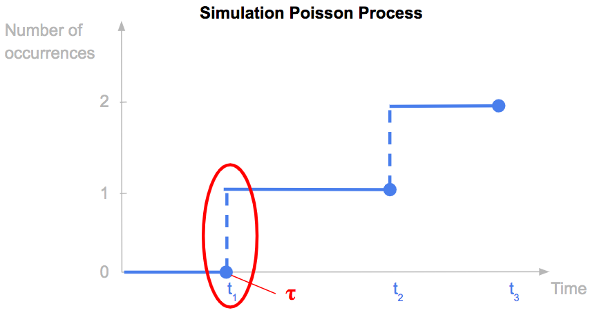
We consider an homogeneous Poisson process N(t) with parameter λ.

N(0) = 0

And the probability to have N(t) = k, so k jump between 0 and t has the following expression. N(t) follows a Poisson(λ.t) distribution.

The default probability between 0 and t is the probability that there is at least one jump in the Poisson process before t.

We recognize the cumulative distribution function of an exponential distribution with parameter λ. The default time 𝛕 follows an exponential distribution.

λ is the default intensity. λ x dt gives the probability that there is a default between t and t+dt knowing that there was no default before t. It is the marginal default probability between t and t+dt.

Proof:

Non-Constant Default Intensity Model

We consider now a non-homogeneous Poisson process N(t) with an intensity (λ_t).

N(0) = 0

The default probability has the following expression, it is a function of the integral of the default intensity between 0 and t.

In this case, the marginal default probability between t and t+dt is given by λ_t x dt.

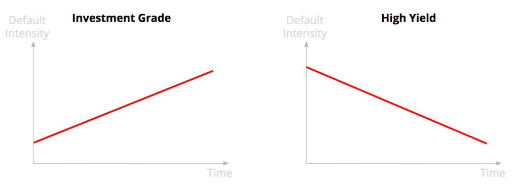
As discussed in another article (link), the evolution of the cumulative and marginal default probabilities depend on the credit quality of the borrower.

For an investment grade borrower with a good credit quality, the default risk is low on the short-term. However if the borrower does not default, there are risks that it will not able to maintain the same credit quality over time, that it downgrades over time meaning an increase of the marginal default probability.

For a high yield borrower with a bad credit quality it is the opposite. Its default probability is high on the short-term. But if it survives it is likely that it upgrades meaning a better credit quality over time and a decrease of the marginal default probability.

Stochastic Default Intensity Model

A Cox process is a Poisson process where the intensity is itself a stochastic process.

In this framework we have:

Duffie and Singleton (1999) uses a Cox-Ingersoll-Ross process for the default intensity:

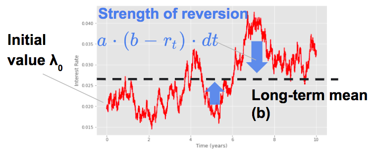
The survival probability S(t) has the following expression in this case. It is similar to the pricing of a zero coupon bond assuming that the short-term interest rate follows a Cox-Ingersoll-Ross process (link).

Watch the Video

More about Credit Risk Modelling

Credit Risk: an Introduction

Credit Risk Modelling: the Probability of Default

Credit Risk Modelling: the Default Time Distribution

Pricing of a Defaultable Bond with a Reduced-Form Model (Part I)

Pricing of a Defaultable Bond with a Reduced-Form Model (Part III, IV, V)

Save 25% on All Quant Next Courses with the Coupon Code: QuantNextBlog25

For students and graduates: We offer a 50% discount on all courses, please contact us if you are interested: contact@quant-next.com

List of Quant Next Courses

We summarize below quantitative finance training courses proposed by Quant Next. Courses are 100% digital, they are composed of many videos, quizzes, applications and tutorials in Python.

Complete training program:

Options, Pricing, and Risk Management Part I: introduction to derivatives, arbitrage free pricing, Black-Scholes model, option Greeks and risk management.

Options, Pricing, and Risk Management Part II: numerical methods for option pricing (Monte Carlo simulations, finite difference methods), replication and risk management of exotic options.

Options, Pricing, and Risk Management Part III:  modelling of the volatility surface,  parametric models with a focus on the SVI model, and stochastic volatility models with a focus on the Heston and the SABR models.

A la carte:

Monte Carlo Simulations for Option Pricing: introduction to Monte Carlo simulations, applications to price options, methods to accelerate computation speed (quasi-Monte Carlo, variance reduction, code optimisation).

Finite Difference Methods for Option Pricing: numerical solving of the Black-Scholes equation, focus on the three main methods: explicit, implicit and Crank-Nicolson.

Replication and Risk Management of Exotic Options: dynamic and static replication methods of exotic options with several concrete examples.

Volatility Surface Parameterization: the SVI Model: introduction on the modelling of the volatility surface implied by option prices, focus on the parametric methods, and particularly on the Stochastic Volatility Inspired (SVI) model and some of its extensions.

The SABR Model: deep dive on on the SABR (Stochastic Alpha Beta Rho) model, one popular stochastic volatility model developed to model the dynamic of the forward price and to price options.

The Heston Model for Option Pricing: deep dive on the Heston model, one of the most popular stochastic volatility model for the pricing of options.