


Volatility & Derivatives
In this post we give an introduction to the Heston model which is one of the most used stochastic volatility model. It assumes that the

The Merton Jump Diffusion model proposed by Merton in 1976 is an extension of the Black-Scholes model (link).
It contains:
μ: annualised expected return on the asset price, σ: annualised volatility of the asset price, Wt: Brownian motion.
Qt: compound Poisson process
Yi: price ratio associated with the i-th jump happening at the random time ti. (Yi) are i.i.d, following a lognormal distribution, and are independent of Wt and Nt, Nt being a Poisson process (link) with intensity λ. E(Qt) = λ.k.t, so Qt – λ.k.t is a martingale.
Reference article: Merton, R. C. (1976) “Option Pricing When underlying stock returns are discontinuous”, Journal of Financial Economics, 3, 125-144
A compound Poisson process is a stochastic process with jumps. The arrival of events (jumps) follows a Poisson process (link). In addition to the random arrival time of events, the magnitude of the jumps is also random, with a specified probability distribution. The magnitudes of the events are independent of each other and also independent of the arrival times.
Example:
λ = 10, T = 1y, jumps ~ N(0, 0.22). 10 jumps per year on average, the magnitude of the jumps follows a normal distribution N(0, 0.22)
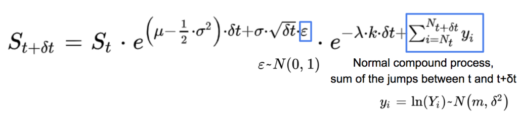
In the Merton Jump Diffusion model, the asset price St follows the SDE:
There is an explicit solution of this SDE1:
1Merton, R. C. (1976) “Option Pricing When underlying stock returns are discontinuous”, Journal of Financial Economics, 3, 125-144
We can simulate the asset price:
S0 = 100, μ = 5%, σ = 20%, λ = 10, T = 5y, jumps ~ N(0, 0.12), δt = 5 / 1000
If there are n jumps between 0 and t, we have:
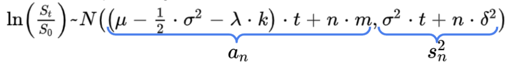
Knowing the number of jumps we can easily deduce the density of ln(St/S0) which follows a normal distribution:
And we obtain the density of ln(St/S0) with the following series using the probability to have n jumps and the conditional distribution:
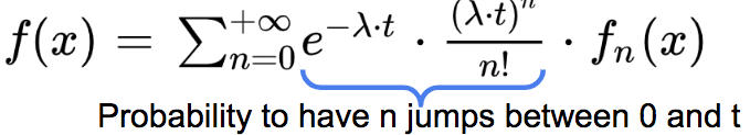
The probability density function of the log-returns is not normal when there are jumps. In addition to an increase of the standard deviation of the log-returns, adding jumps adds tail-risk (kurtosis) and asymmetry (skewness), positive or negative depending on the sign of the average jump.
| Jumps | Distribution jumps | St Deviation | Skewness | Excess Kurtosis |
| No (λ = 0) | + | 0 | 0 | |
| Yes (λ > 0) | m = 0, δ > 0 | ++ | 0 | + |
| Yes (λ > 0) | m > 0, δ > 0 | ++ | + | + |
| Yes (λ > 0) | m < 0, δ > 0 | ++ | – | + |
μ = 5%, σ = 20%, λ = 0 or 1, T = 1y, m = 0 or -0.2, δ = 0.2
Save 25% on All Quant Next Courses with the Coupon Code: QuantNextBlog25
For students and graduates: We offer a 50% discount on all courses, please contact us if you are interested: contact@quant-next.com
We summarize below quantitative finance training courses proposed by Quant Next. Courses are 100% digital, they are composed of many videos, quizzes, applications and tutorials in Python.
Complete training program:
Options, Pricing, and Risk Management Part I: introduction to derivatives, arbitrage free pricing, Black-Scholes model, option Greeks and risk management.
Options, Pricing, and Risk Management Part II: numerical methods for option pricing (Monte Carlo simulations, finite difference methods), replication and risk management of exotic options.
Options, Pricing, and Risk Management Part III: modelling of the volatility surface, parametric models with a focus on the SVI model, and stochastic volatility models with a focus on the Heston and the SABR models.
A la carte:
Monte Carlo Simulations for Option Pricing: introduction to Monte Carlo simulations, applications to price options, methods to accelerate computation speed (quasi-Monte Carlo, variance reduction, code optimisation).
Finite Difference Methods for Option Pricing: numerical solving of the Black-Scholes equation, focus on the three main methods: explicit, implicit and Crank-Nicolson.
Replication and Risk Management of Exotic Options: dynamic and static replication methods of exotic options with several concrete examples.
Volatility Surface Parameterization: the SVI Model: introduction on the modelling of the volatility surface implied by option prices, focus on the parametric methods, and particularly on the Stochastic Volatility Inspired (SVI) model and some of its extensions.
The SABR Model: deep dive on on the SABR (Stochastic Alpha Beta Rho) model, one popular stochastic volatility model developed to model the dynamic of the forward price and to price options.
The Heston Model for Option Pricing: deep dive on the Heston model, one of the most popular stochastic volatility model for the pricing of options.
Import Libraries
import numpy as np
import matplotlib.pyplot as plt
plt.style.use('ggplot')
from scipy.stats import norm
import math
Compound Poisson Process
#Simulate Normal Compound Poisson Process
def normal_compound_poisson_process(lambda_, T, m, delta):

    t = 0
    jumps = 0
    event_values = []
    event_times = []
    event_values.append(0)
    event_times.append(0)
    while t < T:
        t = t + np.random.exponential(1 / lambda_)
        jumps = jumps + np.random.normal(m, delta)
        if t < T:
            event_values.append(jumps)
            event_times.append(t)

    return event_values, event_times

#Plot Normal Compound Poisson Process
def plot_normal_compound_poisson_process(lambda_, T, m, delta):
    event_values, event_times = normal_compound_poisson_process(lambda_, T, m, delta)

    plt.figure(figsize=(10, 8))
    plt.step(event_times, event_values, where='post')
    plt.xlabel('Time (in years)')
    plt.ylabel('Value')
    plt.title('Normal Compound Poisson Process Simulation')
    plt.grid(True)
    plt.show()

#Example
lambda_ = 10  # Intensity of Poisson process
T = 1          # Time
m = .0       # Mean of jumps
delta = .2    # Standard deviation of jumps

plot_normal_compound_poisson_process(lambda_, T, m, delta)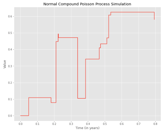
Merton Jump Diffusion Process
#Simulate Merton Jump Diffusion (MJD) Process
def MJD_process(S0, mu, sigma, lambda_, T, m, delta, num_steps):

    dT = T / num_steps
    price = np.zeros(num_steps + 1)
    price[0] = S0
    k = np.exp(m + .5 *delta**2) - 1

    for t in range(1, num_steps + 1):
        # Brownian motion
        Z = np.random.normal(0, 1)
        dW = np.sqrt(dt) * Z
        #jumps between t and t + dt
        jumps = np.sum(normal_compound_poisson_process(lambda_, dT, m, delta)[0])
        price[t] = price[t - 1] * np.exp((r - .5 * sigma**2 - lambda_ * k) * dt + sigma * dW + jumps)

    return price

#Plot Merton Jump Diffusion Process
def plot_MJD_process(S0, mu, sigma, lambda_, T, m, delta, num_steps):

    price_simu = MJD_process(S0, mu, sigma, lambda_, T, m, delta, num_steps)
    time_axis = np.linspace(0, T, num_steps + 1)

    plt.figure(figsize=(10, 5))
    plt.step(time_axis, price_simu, where='post')
    plt.xlabel('Time (in years)')
    plt.ylabel('Price')
    plt.title('Merton Jump Diffusion Process Simulation')
    plt.grid(True)
    plt.show()

#Example
S0 = 100   #initial price
mu = .05   #expected return
sigma = .2   #volatility
lambda_ = 10  # Intensity of Poisson process
T = 5          # Time
m = 0.0       # Mean of jumps
delta = .1    # Standard deviation of jumps
num_steps = 1000 #number of time steps

plot_MJD_process(S0, mu, sigma, lambda_, T, m, delta, num_steps)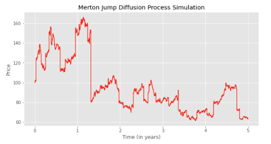
Probability Density Function Log Return with Merton Jump Diffusion Model
#Density Log Return Merton Jump Diffusion (MJD)
def MJD_density(x, mu, sigma, lambda_, T, m, delta, nmax):
    res = 0
    k = np.exp(m + .5 *delta**2) - 1
    for n in range(nmax):
        proba_n = np.exp(-lambda_ * T) * (lambda_ * T)**n / math.factorial(n) #proba n jumps
        a_n = (mu - .5 * sigma**2 - lambda_ * k) * T + n * m #avg conditional normal distribution
        s_n = (sigma**2 * T + n * delta**2)**.5
        res = res + proba_n * norm.pdf(x, a_n, s_n)
    return res

#Plot Density Log Return MJD
def plot_MJD_density(mu, sigma, lambda_, T, m, delta, nmax):
    x = np.linspace(-3., 3., 100)
    params = [mu, sigma, lambda_, T, m, delta, nmax]
    density_x = [MJD_density(x_, *params) for x_ in x]

    plt.figure(figsize=(10, 5))
    plt.plot(x, density_x)
    plt.xlabel('Log Return')
    plt.ylabel('Density')
    plt.title('Density Log Return with Merton Jump Diffusion')
    plt.grid(True)
    plt.show()


#Example
mu = .05   #expected return
sigma = .2   #volatility
lambda_ = 10  # Intensity of Poisson process
T = 1          # Time
m = 0.0       # Mean of jumps
delta = .1    # Standard deviation of jumps
nmax = 100 #maximum number of jumps

plot_MJD_density(mu, sigma, lambda_, T, m, delta, nmax)
#Example
mu = .05 #expected return
sigma = .2 #volatility
#lambda_ = 10 # Intensity of Poisson process
T = 1 # Time
m = 0.0 # Mean of jumps
delta = .2 # Standard deviation of jumps
nmax = 100 #maximum number of jumps
x = np.linspace(-3., 3., 100)
params0 = [mu, sigma, 0, T, m, delta, nmax]
params1 = [mu, sigma, 1, T, m, delta, nmax]
params2 = [mu, sigma, 1, T, -0.2, delta, nmax]
density_x0 = [MJD_density(x_, *params0) for x_ in x]
density_x1 = [MJD_density(x_, *params1) for x_ in x]
density_x2 = [MJD_density(x_, *params2) for x_ in x]
plt.figure(figsize=(10, 5))
plt.plot(x, density_x0, label = 'Normal Distribution (No Jumps)')
plt.plot(x, density_x1, label = 'Distribution with Jumps')
plt.plot(x, density_x2, label = 'Distribution with Jumps, m < 0')
plt.xlabel('Log Return')
plt.ylabel('Density')
plt.title('Density Log Return with Merton Jump Diffusion')
plt.grid(True)
plt.legend()
plt.show()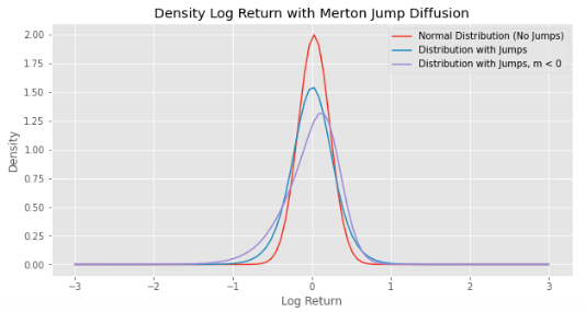
In this post we give an introduction to the Heston model which is one of the most used stochastic volatility model. It assumes that the

In the previous post (link) dedicated to the pricing of defaultable bonds with a reduced form model, we saw how to price a zero coupon

The Merton Jump Diffusion (MJD) model was introduced in a previous article (link). It is an extension of the Black-Scholes model adding a jump part