The Heston Model: an Introduction

In this post we give an introduction to the Heston model which is one of the most used stochastic volatility model. It assumes that the variance is stochastic, it is correlated with the asset price and follows a mean-reverting Cox Ingersoll Ross (CIR) process.

Limits of the Black-Scholes model

In the Black-Scholes model, the asset price is assumed to follow a geometric Brownian motion.

The implied volatility is assume to be constant, this not true in practice the volatility changes with time. 

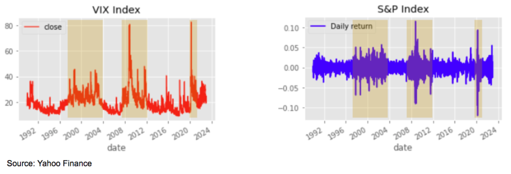
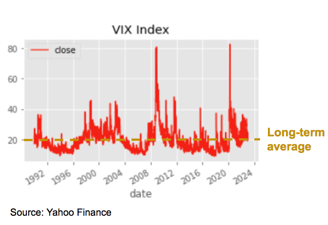
The chart below shows the historical time series of the volatility index VIX from 1990 to 2022. the VIX index is a measure of the expected volatility of the US stock market over the next 30 days derived from S&P 500 options.

Source: Yahoo Finance

The next chart represents the historical daily change of the S&P over the same period of time.

Source: Yahoo Finance

The volatility clusters and reverts to its mean

The volatility clusters, large (resp. small) movements are in general followed by large (resp. small) movements.

We also observe that after periods of large fluctuations and high volatility, when there is an improvement of the market sentiment, the volatility tends to go back to normal levels. The long-term average is typically close to 20 for the VIX index.

Equities and volatilities are negatively correlated in general

Negative stock returns tend to be associated with higher volatility, and we observe a negative correlation between stock returns and volatility changes in general. 

There are two main explanations for this in the literature.

On the one hand, when a stock goes down, the leverage of the company increases making its equity more volatile. This is the so-called leverage effect. 

On the other hand, persistent high volatility can cause stock prices to drop with the selling of risky assets and flight to safety by risk-averse asset managers.

Source: Yahoo Finance

The Heston model

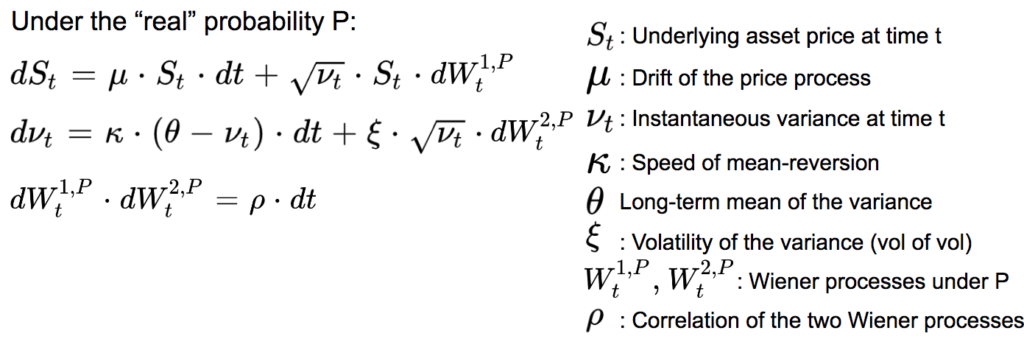
Heston proposed in 1993 a model to value options where Both the asset price and the volatility are stochastic. The volatility follows a mean-reverting process, the asset price and its volatility are correlated.

Under the real probability P, the asset price, follows a process close to geometric brownian motion with mu the drift of the price process. But the instantaneous volatility, the square root of the instantaneous variance is stochastic as well.

Reference article: Heston, Steven L. (1993), “A closed-form  solution for options with stochastic volatility with applications to bond and currency options”.

The variance follows a mean-reverting process…

In the Heston model, the instantaneous variance follows a Cox-Ingersoll-Ross mean-reverting process. Here is a simulation of a volatility path with the Cox-Ingersoll-Ross model.

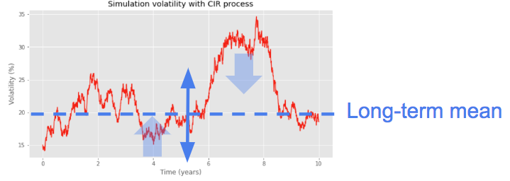
κ controls the speed of mean-reversion of the process. It represents the velocity at which the process will revert to its mean. θ is the long-term mean of the variance.

When the distance to the mean is high, the strength of mean-reversion will be high a well, with a strong opposite force pushing the trajectory back to its mean. The higher the kappa or the distance to the mean, the stronger the mean-reversion force.

The volatility of the variance ξ, also called vol of vol, controls the amplitude of the possible fluctuations around the mean.

If 2 x κ x θ > ξ, then the instantaneous variance is strictly positive. This is known as the Feller condition.

More about the Cox-Ingersoll-Ross process: The Cox-Ingersoll-Ross (CIR) Model

… and is correlated with the asset price

In the Heston model, the randomness of the asset price and its variance are controlled by two correlated wiener processes.

The correlation parameter ρ controls the relationship between the dynamic of the underlying asset price and its volatility.

ρ will be typically negative for stocks.

Parameters in the Heston model

So in addition to the drift of the asset price process, the Heston model has five unknown parameters:

• ν₀: the initial level of the variance,

• κ: the speed of reversion of the variance process,

• θ: the long term mean of the variance,

• ξ: the volatility of the variance or vol of vol,

• ρ: the correlation between the stock price and its variance.

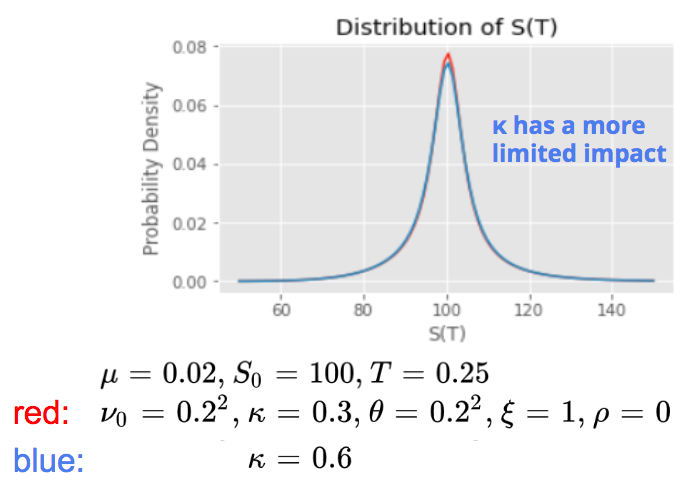
We will now simulate the distribution of the asset price at a time horizon of one quarter, changing the different parameters.

First we assume that the correlation and the vol of vol parameters are equal to zero. The volatility is deterministic in this case. We assume that it is constant, equal to 0.2 on an annualised basis. The initial variance and the long-term variance are both equal to the square of 0.2. We are back in the Black-Scholes framework, the log return follows a gaussian distribution.

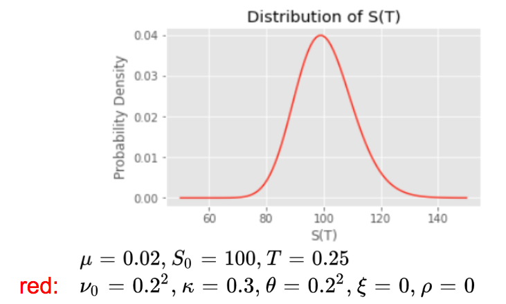
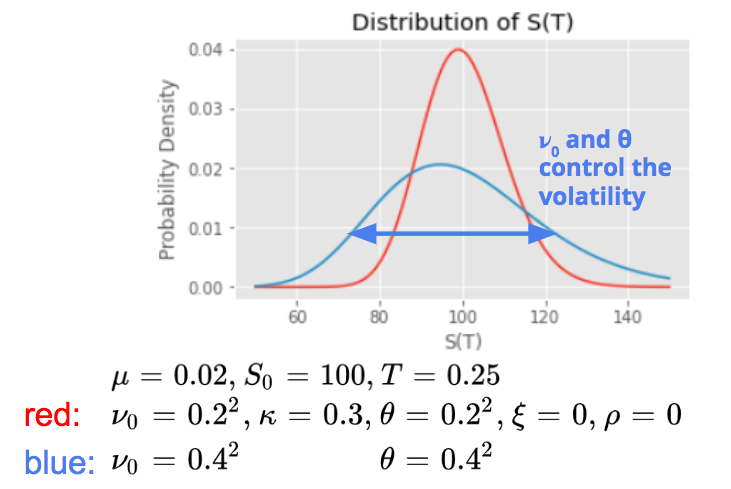
The initial variance ν₀ and the long term variance θ both control the volatility of the asset price return.

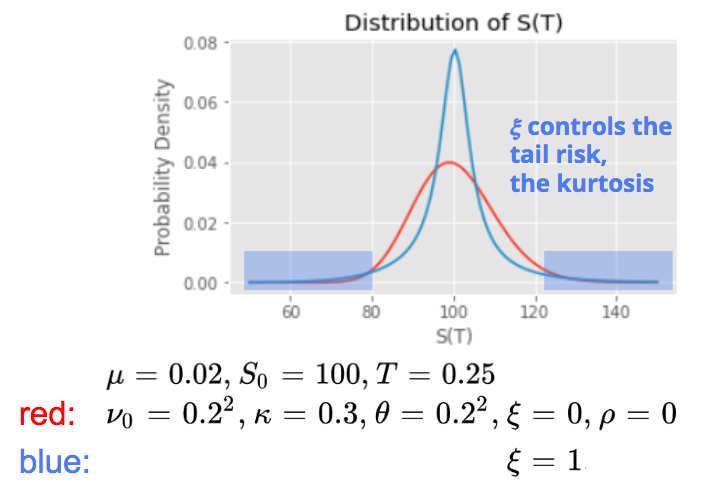
The vol of vol ξ controls the tail risk, the kurtosis of the distribution. A higher vol of vol will increase the probability to have extreme movements on both sides, the distribution is no more gaussian, it has fatter tails.

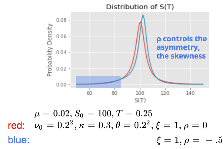
The correlation parameter ρ controls the asymmetry of the distribution, its skewness. A very negative correlation, like what we observe in general on the equity market, would increase the probability to have very negative returns, with higher fluctuations on the downside. 

The speed of reversion κ has a more limited impact on the asset price distribution.

In practice, this parameter is often fixed, all other being enough to calibrate the model.

This parameter can be better interpreted with the concept of half-life, the ‘half life’ is the average time it will take to get half-way back to the mean which can be calculated from the ratio between log(2) and kappa.

Half-life = ln(2) / κ

For example, if the mean reversion coefficient kappa is equal to 0.3, then the half-life of the process is close to 2.3 years. A higher kappa will reduce the half-life, as it will increase the speed of reversion.

Save 25% on All Quant Next Courses with the Coupon Code: QuantNextBlog25

For students and graduates: We offer a 50% discount on all courses, please contact us if you are interested: contact@quant-next.com

List of Quant Next Courses

We summarize below quantitative finance training courses proposed by Quant Next. Courses are 100% digital, they are composed of many videos, quizzes, applications and tutorials in Python.

Complete training program:

Options, Pricing, and Risk Management Part I: introduction to derivatives, arbitrage free pricing, Black-Scholes model, option Greeks and risk management.

Options, Pricing, and Risk Management Part II: numerical methods for option pricing (Monte Carlo simulations, finite difference methods), replication and risk management of exotic options.

Options, Pricing, and Risk Management Part III:  modelling of the volatility surface,  parametric models with a focus on the SVI model, and stochastic volatility models with a focus on the Heston and the SABR models.

A la carte:

Monte Carlo Simulations for Option Pricing: introduction to Monte Carlo simulations, applications to price options, methods to accelerate computation speed (quasi-Monte Carlo, variance reduction, code optimisation).

Finite Difference Methods for Option Pricing: numerical solving of the Black-Scholes equation, focus on the three main methods: explicit, implicit and Crank-Nicolson.

Replication and Risk Management of Exotic Options: dynamic and static replication methods of exotic options with several concrete examples.

Volatility Surface Parameterization: the SVI Model: introduction on the modelling of the volatility surface implied by option prices, focus on the parametric methods, and particularly on the Stochastic Volatility Inspired (SVI) model and some of its extensions.

The SABR Model: deep dive on on the SABR (Stochastic Alpha Beta Rho) model, one popular stochastic volatility model developed to model the dynamic of the forward price and to price options.

The Heston Model for Option Pricing: deep dive on the Heston model, one of the most popular stochastic volatility model for the pricing of options.