Options, Greeks and P&L Decomposition (Part 3)

In previous articles (see Options, Greeks and P&L Decomposition (Part 1) and Options, Greeks and P&L Decomposition (Part 2)) we decomposed the P&L of simple option strategies in different time horizons with the major first and second order greeks.

In this article, we analyse the P&L of a short iron butterfly option strategy, which is a combination of a long straddle and a short strangle strategies, on a short period of time.

We show that the P&L of the strategy is mostly explained by the vega and the volga risks. While the vega risk can be managed by adjusting the long / short quantities, the strategy remains exposed to the volga risk which is higher on the wings.

The Python code used in simulations is available at the end of the article.

P&L Decomposition of the Strategy

The P&L of an option strategy between t and t+δt can be decomposed with the different first order and second order Greeks:

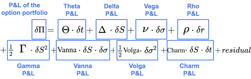
Theta, delta, vega, rho are the first order Greeks:

• The theta or time decay measures the rate at which the value of the option declines due to the passage of time.
• The delta of an option measures the change in the option’s price resulting from a change in the underlying asset. For option traders, minus delta indicates how many underlying assets are needed to be purchased or sold to hedge the directional exposure of the option position.
• Vega measures the change in the option’s price resulting from a change in the implied volatility.
• Rho measures the option’s sensitivity to changes in the risk-free rate of interest.

On the second line are the most important second order Greeks:

• The gamma measures the rate of change of the delta of an option relative to the underlying asset price. It is the second order partial derivative of the value of the option with respect to the price of the underlying asset.
• The Vanna measures the option’s sensitivity to small changes in the underlying asset price and volatility.  It is the sensitivity of the delta to changes in the volatility or the sensitivity of the vega to changes in the underlying asset price.
• The volga or vomma measures the sensitivity of the vega to a change in the implied volatility.  It is the second order partial derivative of the price of the option with respect to the implied volatility.
• The charm is the option’s sensitivity to small changes in the underlying asset price and passage of time. It is also the sensitivity of the delta to the passage of time or the sensitivity of the theta to changes in the underlying asset price.

The residual regroups other second order and higher order sensitivities.

Short Iron Butterfly Strategy

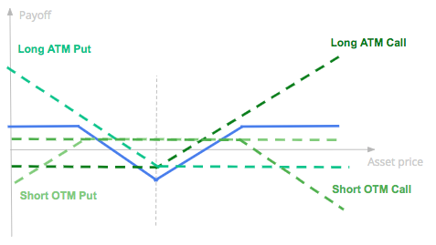
A short iron butterfly strategy consists on:

• the purchase of a straddle, long at-the-money (ATM) call and put
• and the selling of a strangle, short out-of-the-money (OTM) call and put

Such strategy will generate some profits at the maturity of the option if there is an important movement of the underlying asset price both on the downside or on the upside, but the investor is not expecting too high movements as he is selling OTM call and put to finance a part of the purchase of ATM options.

Payoff of a Short Iron Butterfly

In terms of Greeks, a short iron butterfly has:

• a close to zero delta: both the long straddle and the short strangle have a close to zero directional exposure to the underlying asset price.
• A positive gamma: the convexity is maximum ATM, the positive gamma of the long straddle is higher than the negative gamma of the short strangle.
• A negative theta: the positive gamma comes with a negative time value, the cost of the purchase of ATM options is higher than the premium received for selling OTM ones.
• A positive vega: the vega is the highest when options are ATM, resulting in a positive vega exposure of the long straddle / short strangle strategy.
• A close to zero vanna: the vanna is positive in general for a long OTM call option while it is negative for a long OTM put option, it is close to zero for ATM options. Both the long straddle and the short strangle have a low vanna exposure. A higher volatility means a higher delta for an OTM call and a lower delta for an OTM put as it becomes more likely when the volatility increases that the option moves in the money and that the delta becomes more positive for call options and more negative for put options. The delta of ATM options is less sensitive to volatility changes.
• A negative volga: on the other hand, the volga risk, or vol of vol risk is attributed to the wings. Long OTM options, both calls and puts, have a positive volga exposure, while ATM options have a close to zero one. This results in a negative volga exposure of the short iron butterfly which combines a long straddle (close to zero volga) with a short strangle (negative volga). The vega is higher for ATM options than for OTM ones. However, an OTM option will be more similar to an ATM one when the implied volatility increases, as it becomes more likely to be exercised. So the vega of an OTM option increases with implied volatility, meaning a positive volga.

Case Studies

We will decompose the P&L of a short iron butterfly strategy on a weekly time horizon with different scenarios using these six greeks.

We assume that we are in the Black-Scholes framework, the implied volatility is constant.

Below are the characteristics of the strategy and the market parameters.

#parameters
S0 = 100 #stock price
Kputstraddle = 100 #strike price put long straddle
Kcallstraddle = 100 #strike price call long straddle
Kputstrangle = 95 #strike price put short strangle
Kcallstrangle = 105 #strike price call short strangle
r = .0 #risk-free interest rate
q = .0 #dividend yield
T0 = 21 / 252 #time to maturity
sigma0 = 0.3 #implied volatility BS
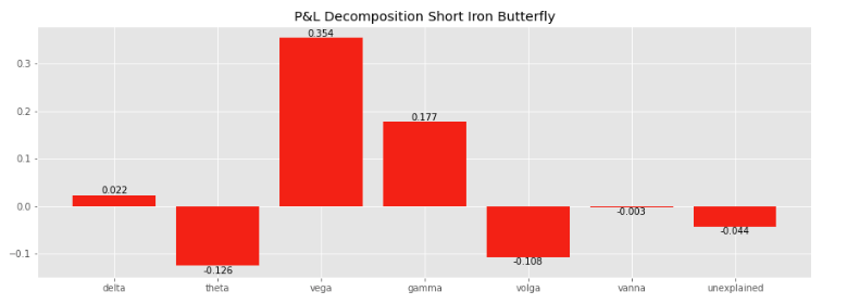
dt = 5 / 252 #5bd

1/ Stock Price: -5%, Volatility : + 10% in one week

In this first case study, we assume that the stock price goes down by -5% while the implied volatility goes up by +10% in a weekly horizon. We also assume that an equal number of options are bought and sold (1).

dS = -100 * 0.05 #stock movement
dsigma = +0.1 #implied volatility movement
ratio = 1 #if ratio = 1: same number of options are bought and sold

As highlighted in the chart below, the strategy would have performed positively, benefiting mostly from the rise of volatility with its positive vega exposure.

The positive gamma of the short iron butterfly strategy is partly offset by its negative theta, but gamma + theta remains positive in this scenario, the realised volatility being higher than the implied one.

The volga has a negative contribution. As said before, the volga of the strategy, which is selling the wings via the short strangle position, is negative.

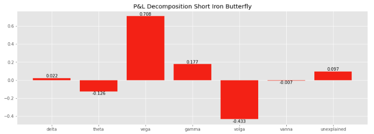
2/ Stock Price: -5%, Volatility + 20% in one week

In this second case study, we assume that the implied volatility increases by +20% from 30% to 50%, while we still assume a decline of -5% of the stock price in a week. We still assume as well that an equal number of options are bought and sold in the butterfly strategy (1).

dS = -100 * 0.05 #stock movement
dsigma = +0.2 #implied volatility movement
ratio = 1 #if ratio = 1: same number of options are bought and sold

The vega P&L is multiplied by two, in line with the higher movement of the implied volatility, while the volga P&L is multiplied by four, explaining a more important part of the P&L of the strategy which remains positive in this second scenario.

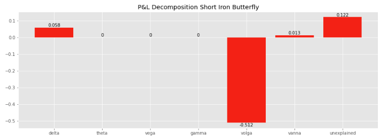
3/ Stock Price: -5%, Volatility + 20% in one week, vega-hedged strategy

In this third case study, we assume that weekly market movements are the same as in the previous: -5% for the stock price, +20% for the implied volatility.

We assume now that the strategy is vega-neutral, we sell more strangle (1.2x) in front of the straddle in order to cancel the vega exposure.

dS = -100 * 0.05 #stock movement
dsigma = +0.2 #implied volatility movement
ratio = (EuropeanOptionBS(S0, Kputstraddle, T0, r, q, sigma0, "Call").vega \
    + EuropeanOptionBS(S0, Kcallstraddle, T0, r, q, sigma0, "Put").vega) \
    / (EuropeanOptionBS(S0, Kputstrangle, T0, r, q, sigma0 + smile, "Call").vega \
     + EuropeanOptionBS(S0, Kcallstrangle, T0, r, q, sigma0 + smile, "Put").vega) 
#ratio: number of strangle to be sold in front of the straddle to be vega-neutral

By doing that, we see that the strategy is gamma-neutral in addition to be vega-neutral, the ratio of the vega being the same as the ratio of the gamma.

On the other hand, we are not able to cancel the volga exposure. On the contrary, the negative contribution of the volga is even greater by increasing the number of OTM options we sell. The P&L of the strategy is now negative, mostly explained by its volga.

Save 10% on All Quant Next Courses with the Coupon Code: QuantNextBlog10

For students and graduates: We offer a 50% discount on all courses, please contact us if you are interested: contact@quant-next.com

Python Code

First we import the libraries that will be used and we create a class EuropeanOptionBS with Black-Scholes prices and Greeks with closed-form formulas.

#import libraries
import matplotlib.pyplot as plt
plt.style.use('ggplot')
import math
import numpy as np
import pandas as pd
from scipy.stats import norm
%matplotlib inline

#Black-Scholes price and Greeks
class EuropeanOptionBS:

    def __init__(self, S, K, T, r, q, sigma, Type):
        self.S = S
        self.K = K
        self.T = T
        self.r = r
        self.q = q        
        self.sigma = sigma
        self.Type = Type
        self.d1 = self.d1()
        self.d2 = self.d2()
        self.price = self.price()
        self.delta = self.delta()
        self.theta = self.theta()
        self.vega = self.vega()
        self.gamma = self.gamma()
        self.volga = self.volga()
        self.vanna = self.vanna()        
        
    def d1(self):
        d1 = (math.log(self.S / self.K) \
                   + (self.r - self.q + .5 * (self.sigma ** 2)) * self.T) \
                    / (self.sigma * self.T ** .5)       
        return d1

    def d2(self):
        d2 = self.d1 - self.sigma * self.T ** .5     
        return d2
    
    def price(self):
        if self.Type == "Call":
            price = self.S * math.exp(-self.q * self.T) * norm.cdf(self.d1) \
            - self.K * math.exp(-self.r * self.T) * norm.cdf(self.d2)
        if self.Type == "Put":
            price = self.K * math.exp(-self.r * self.T) * norm.cdf(-self.d2) \
            - self.S * math.exp(-self.q * self.T) * norm.cdf(-self.d1)            
        return price
    
    def delta(self):
        if self.Type == "Call":
            delta = math.exp(-self.q * self.T) * norm.cdf(self.d1)
        if self.Type == "Put":
            delta = -math.exp(-self.q * self.T) * norm.cdf(-self.d1)
        return delta
    
    def theta(self):
        if self.Type == "Call":
            theta1 = -math.exp(-self.q * self.T) * \
            (self.S * norm.pdf(self.d1) * self.sigma) / (2 * self.T ** .5)
            theta2 = self.q * self.S * math.exp(-self.q * self.T) * norm.cdf(self.d1)
            theta3 = -self.r * self.K * math.exp(-self.r * self.T) * norm.cdf(self.d2)
            theta = theta1 + theta2 + theta3
        if self.Type == "Put":
            theta1 = -math.exp(-self.q * self.T) * \
            (self.S * norm.pdf(self.d1) * self.sigma) / (2 * self.T ** .5)
            theta2 = -self.q * self.S * math.exp(-self.q * self.T) * norm.cdf(-self.d1)
            theta3 = self.r * self.K * math.exp(-self.r * self.T) * norm.cdf(-self.d2)
            theta =  theta1 + theta2 + theta3
        return theta
    
    def vega(self):
        vega = self.S * math.exp(-self.q * self.T) * self.T** .5 * norm.pdf(self.d1)
        return vega
    
    def gamma(self):
        gamma = math.exp(-self.q * self.T) * norm.pdf(self.d1) / (self.S * self.sigma * self.T** .5)
        return gamma
    
    def volga(self):
        volga = self.vega / self.sigma * self.d1 * self.d2
        return volga
    
    def vanna(self):
        vanna = -self.vega / (self.S * self.sigma * self.T** .5) * self.d2
        return vanna

Then we enter the parameters, we give one example of set of parameters here.

#parameters
S0 = 100 #stock price
Kputstraddle = 100 #strike price put straddle
Kcallstraddle = 100 #strike price call straddle
Kputstrangle = 95 #strike price put strangle
Kcallstrangle = 105 #strike price call strangle
r = .0 #risk-free interest rate
q = .0 #dividend
T0 = 21 / 252 #time to maturity
sigma0 = 0.3 #implied volatility BS
dt = 5 / 252 #5bd
smile = 0.#vol_Kcall - vol_Kput
ratio = (EuropeanOptionBS(S0, Kputstraddle, T0, r, q, sigma0, "Call").vega \
    + EuropeanOptionBS(S0, Kcallstraddle, T0, r, q, sigma0, "Put").vega) \
    / (EuropeanOptionBS(S0, Kputstrangle, T0, r, q, sigma0 + smile, "Call").vega \
     + EuropeanOptionBS(S0, Kcallstrangle, T0, r, q, sigma0 + smile, "Put").vega) 
#ratio: number of strangle to be sold in front of the straddle to be vega-neutral 
#ratio = 1 #if ratio = 1: same number of options are bought and sold
#Market changes between t and t+dt
dS = -100 * 0.05 #stock movement
dsigma = +0.2 #implied volatility movement
T1 = T0 - dt #time to maturity
S1 = S0 + dS #new stock price
sigma1 = sigma0 + dsigma #new implied volatility

We calculate the P&L between t and t + δt.

#P&L of the strategy
P0 = EuropeanOptionBS(S0, Kputstraddle, T0, r, q, sigma0, "Call").price \
    + EuropeanOptionBS(S0, Kcallstraddle, T0, r, q, sigma0, "Put").price \
    - (EuropeanOptionBS(S0, Kputstrangle, T0, r, q, sigma0 + smile, "Call").price \
     + EuropeanOptionBS(S0, Kcallstrangle, T0, r, q, sigma0 + smile, "Put").price) * ratio
P1 = EuropeanOptionBS(S0, Kputstraddle, T0, r, q, sigma1, "Call").price \
    + EuropeanOptionBS(S0, Kcallstraddle, T0, r, q, sigma1, "Put").price \
    - (EuropeanOptionBS(S0, Kputstrangle, T0, r, q, sigma1 + smile, "Call").price \
     + EuropeanOptionBS(S0, Kcallstrangle, T0, r, q, sigma1 + smile, "Put").price) * ratio
delta0 = EuropeanOptionBS(S0, Kputstraddle, T0, r, q, sigma0, "Call").delta \
    + EuropeanOptionBS(S0, Kcallstraddle, T0, r, q, sigma0, "Put").delta \
    - (EuropeanOptionBS(S0, Kputstrangle, T0, r, q, sigma0 + smile, "Call").delta \
     + EuropeanOptionBS(S0, Kcallstrangle, T0, r, q, sigma0 + smile, "Put").delta) * ratio
isDeltaHedged = 0 #1 if is delta-hedged, 0 otherwise
dPandL = P1 - P0 - delta0 * dS * isDeltaHedged
print("P&L: " + str(dPandL))

We decompose the P&L between the contribution of the different Greeks and we plot it with a barchart.

#initial greeks
delta0 = EuropeanOptionBS(S0, Kputstraddle, T0, r, q, sigma0, "Call").delta \
    + EuropeanOptionBS(S0, Kcallstraddle, T0, r, q, sigma0, "Put").delta \
    - (EuropeanOptionBS(S0, Kputstrangle, T0, r, q, sigma0 + smile, "Call").delta \
     + EuropeanOptionBS(S0, Kcallstrangle, T0, r, q, sigma0 + smile, "Put").delta) * ratio
theta0 = EuropeanOptionBS(S0, Kputstraddle, T0, r, q, sigma0, "Call").theta \
    + EuropeanOptionBS(S0, Kcallstraddle, T0, r, q, sigma0, "Put").theta \
    - (EuropeanOptionBS(S0, Kputstrangle, T0, r, q, sigma0 + smile, "Call").theta \
     + EuropeanOptionBS(S0, Kcallstrangle, T0, r, q, sigma0 + smile, "Put").theta) * ratio
vega0 = EuropeanOptionBS(S0, Kputstraddle, T0, r, q, sigma0, "Call").vega \
    + EuropeanOptionBS(S0, Kcallstraddle, T0, r, q, sigma0, "Put").vega \
    - (EuropeanOptionBS(S0, Kputstrangle, T0, r, q, sigma0 + smile, "Call").vega \
     + EuropeanOptionBS(S0, Kcallstrangle, T0, r, q, sigma0 + smile, "Put").vega) * ratio
gamma0 = EuropeanOptionBS(S0, Kputstraddle, T0, r, q, sigma0, "Call").gamma \
    + EuropeanOptionBS(S0, Kcallstraddle, T0, r, q, sigma0, "Put").gamma \
    - (EuropeanOptionBS(S0, Kputstrangle, T0, r, q, sigma0 + smile, "Call").gamma \
     + EuropeanOptionBS(S0, Kcallstrangle, T0, r, q, sigma0 + smile, "Put").gamma) * ratio
volga0 = EuropeanOptionBS(S0, Kputstraddle, T0, r, q, sigma0, "Call").volga \
    + EuropeanOptionBS(S0, Kcallstraddle, T0, r, q, sigma0, "Put").volga \
    - (EuropeanOptionBS(S0, Kputstrangle, T0, r, q, sigma0 + smile, "Call").volga \
     + EuropeanOptionBS(S0, Kcallstrangle, T0, r, q, sigma0 + smile, "Put").volga) * ratio
vanna0 = EuropeanOptionBS(S0, Kputstraddle, T0, r, q, sigma0, "Call").vanna \
    + EuropeanOptionBS(S0, Kcallstraddle, T0, r, q, sigma0, "Put").vanna \
    - (EuropeanOptionBS(S0, Kputstrangle, T0, r, q, sigma0 + smile, "Call").vanna \
     + EuropeanOptionBS(S0, Kcallstrangle, T0, r, q, sigma0 + smile, "Put").vanna) * ratio

#P&L attribution
delta_PandL = delta0 * dS * (1 - isDeltaHedged)
theta_PandL = theta0 * dt
vega_PandL = vega0 * dsigma
gamma_PandL = 1 / 2 * gamma0 * dS**2
volga_PandL = 1 / 2 * volga0 * dsigma**2
vanna_PandL = vanna0 * dS * dsigma
unexplained = dPandL - sum([delta_PandL, theta_PandL, vega_PandL, gamma_PandL, volga_PandL, vanna_PandL])
y = [delta_PandL, theta_PandL, vega_PandL, gamma_PandL, volga_PandL, vanna_PandL, unexplained]
x = ["delta", "theta", "vega", "gamma", "volga", "vanna","unexplained"]

fig, ax = plt.subplots(figsize = (15,5))
bars = ax.bar(x, np.round(y,3))
plt.title("P&L Decomposition Short Iron Butterfly")
ax.bar_label(bars)
plt.show();