Options, Greeks and P&L Decomposition (Part 2)

In a previous article (see Options, Greeks and P&L Decomposition (Part 1)) we analysed the decomposition of the P&L of an option strategy in a short period of time with the major first and second order greeks.

In this new article, we assume that the option is kept for a certain period of time, delta-hedged regularly, and we study the P&L of the strategy in theory and in practice through simulations.

We show that under certain assumptions, the P&L of a delta-hedged option is mostly explained by the gamma / theta P&L when the option is kept until expiry, it is not depending on the path of the implied volatility.

The Python code used in simulations is available at the end of the article.

P&L Decomposition

We consider a delta-hedged option strategy consisting on:

• The purchase of one option: P
• The selling of Δ stocks to offset the delta risk with the Black-Scholes delta: -Δ.S
• The borrow in cash of -P + Δ.S to finance the strategy

We assume that there are no transaction costs, the risk-free interest rate and the dividend yield are constant equal to r and q respectively.

The P&L of the strategy between t and t + δt is equal to:

Equation 1

P = P(t, S, σ) is the Black-Scholes price of the option.

With a Taylor expansion of the option price we have:

Equation 2

with Δ: delta, Γ: gamma, Θ: theta, v: vega of the option.

And P is solution of the Black-Scholes equation, so we have the following relationship between the theta (Θ) and the gamma (Γ) of the option:

Equation 3

Replacing Θ in Equation 2 with its expression from Equation 3 and δP in Equation 1 with its expression from Equation 2 we get the following expression for the P&L of the strategy between t and t + δt:

Equation 4

with σ_r the realised volatility:

So if we neglect other higher order greeks such as vanna, volga, charm and so on, the P&L of the strategy between t and t + δt is mostly explained by

• The gamma / theta P&L:

• The vega P&L:

If we maintain the strategy for a certain time, with a regular delta-hedging, the P&L of the strategy will be path-dependent, the gamma and the vega of the option with change with the moneyness of the option, its time to maturity or the implied volatility.

Going back to Equation 1, if we neglect interest rates and dividends and we assume that we delta-hedge the option regularly using the implied volatility at inception, the P&L between t₀ and t₁ is:

Equation 6

If we consider a European vanilla option such as a call option and we assume that the option is kept until expiry, we see that the P&L of the strategy is no more depending on the implied volatility path. The price of the option at expiry T is its final payoff (S_T – K)⁺ with K the strike price of the option, and the P&L becomes:

Equation 7

If the option is delta-hedged with a high enough frequency, the P&L at expiry of the delta-hedged option is actually very close to the gamma / theta P&L by integrating Equation 4 without the vega term and the residual.

Equation 8

Let’s test it through simulations.

Market Simulations

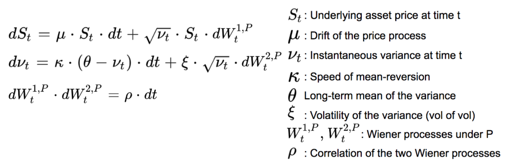
We assume that the stock price follows a Heston model.

Both the stock price and its volatility are stochastic. Under the real probability P we have:

The Heston Model

Equation 8

We use the following Euler discretization for the simulations, using the full truncation method scheme replacing nu by the maximum between 0 and nu in the mean reversion term, in the square root of the variance and in the asset price expression:

Equation 9

References: Roger Lord, Remmert Koekkoek, Dick van Dijk (2008) “A comparison of biased simulation schemes for stochastic volatility models”

N₁ and N₂ are independent random variable, they follow a standard normal distribution.

In order to simulate the implied volatility, we assume that the implied variance (the square of the implied volatility) is equal to the instantaneous variance plus a certain variance premium p:

Equation 10

We use the following parameters and run 100 simulations:

S₀ = 100, ν₀ = 0.2², μ = 5%, κ = 5, θ = 0.2², ξ = 0.5, ρ = -50%, p = 0.3² – 0.2²

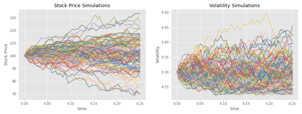
And we consider the two following simulations with a 3-month horizon:

Simulation 1: stock price up / vol down

Simulation 2: stock price down / vol up

P&L Simulations

We consider a 3-month call option with a strike price at 105, and we price the option with the Black-Scholes formula assuming the risk-free interest rate r = 3% and the dividend yield q = 0%.

The strategy consists on the purchase of the option, it is delta-hedged on a daily basis using the volatility at inception until the maturity of the option.

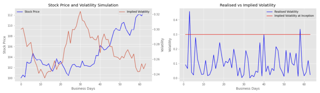
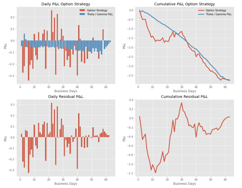
As highlighted below, in Simulation 1 (stock price up / vol down) , the P&L of the strategy is negative at maturity. The realised volatility (see above) is most of the time below the implied volatility, and the gamma / theta P&L has a negative contribution. At maturity, most of the P&L is explained by the Theta / Gamma P&L, the cumulative residual P&L, mostly explained by the Vega P&L, is close to zero at the maturity of the option.

P&L Option Strategy – Simulation 1

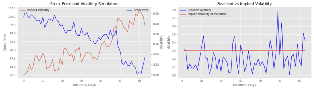
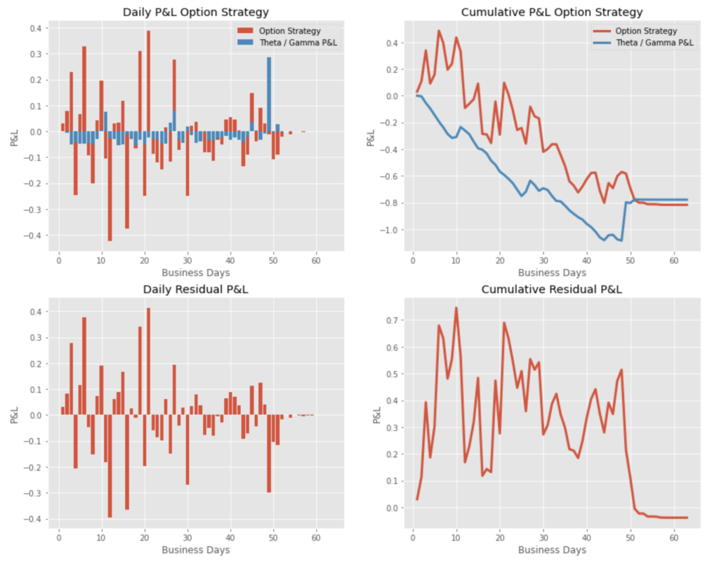
In Simulation 2 (stock price down, vol up), the P&L is a bit less negative. The realized volatility is a bit less below the implied volatility at inception (see above). Again, most of the P&L at maturity is explained by the Theta / Gamma P&L, the cumulative residual P&L converging to a value close to zero.

P&L Option Strategy – Simulation 2

In both cases, the P&L is no more directional, as the option is delta-hedged.

Even if the volatility P&L (vega, vanna, volga, …) can have important impact on the daily P&L, when the option is kept until expiry, it cancels out cumulatively and the final P&L is mostly explained by the gamma / theta P&L.

Save 10% on All Quant Next Courses with the Coupon Code: QuantNextBlog10

For students and graduates: We offer a 50% discount on all courses, please contact us if you are interested: contact@quant-next.com

Python Code

First we import the libraries that will be used and we create a class EuropeanOptionBS with Black-Scholes prices and Greeks with closed-form formulas.

Import Libraries:

import matplotlib.pyplot as plt
plt.style.use('ggplot')
import math
import numpy as np
import pandas as pd
from scipy.stats import norm
%matplotlib inline

Black-Scholes formula and greeks:

class EuropeanOptionBS:

    def __init__(self, S, K, T, r, q, sigma, Type):
        self.S = S
        self.K = K
        self.T = T
        self.r = r
        self.q = q        
        self.sigma = sigma
        self.Type = Type
        self.d1 = self.d1()
        self.d2 = self.d2()
        self.price = self.price()
        self.delta = self.delta()
        self.theta = self.theta()
        self.vega = self.vega()
        self.gamma = self.gamma()
        self.volga = self.volga()
        self.vanna = self.vanna()        

    def d1(self):
        d1 = (math.log(self.S / self.K) \
               + (self.r - self.q + .5 * (self.sigma ** 2)) * self.T) \
                / (self.sigma * self.T **.5)       
        return d1

    def d2(self):
        d2 = self.d1 - self.sigma * self.T **.5     
        return d2

    def price(self):
        if self.Type == "Call":
            price = self.S * math.exp(-self.q * self.T) * norm.cdf(self.d1) \
            - self.K * math.exp(-self.r * self.T) * norm.cdf(self.d2)
        if self.Type == "Put":
            price = self.K * math.exp(-self.r* self.T) * norm.cdf(-self.d2) \
            - self.S * math.exp(-self.q * self.T) * norm.cdf(-self.d1)            
        return price

    def delta(self):
        if self.Type == "Call":
            delta = math.exp(-self.q * self.T) * norm.cdf(self.d1)
        if self.Type == "Put":
            delta = -math.exp(-self.q * self.T) * norm.cdf(-self.d1)
        return delta

    def theta(self):
        if self.Type == "Call":
            theta1 = -math.exp(-self.q * self.T) * \
            (self.S * norm.pdf(self.d1) * self.sigma) / (2 * self.T**.5)
            theta2 = self.q * self.S * math.exp(-self.q * self.T) * norm.cdf(self.d1)
            theta3 = -self.r * self.K * math.exp(-self.r * self.T) * norm.cdf(self.d2)
            theta = theta1 + theta2 + theta3
        if self.Type == "Put":
            theta1 = -math.exp(-self.q * self.T) * \
            (self.S * norm.pdf(self.d1) * self.sigma) / (2 * self.T **.5)
            theta2 = -self.q * self.S * math.exp(-self.q * self.T) * norm.cdf(-self.d1)
            theta3 = self.r * self.K * math.exp(-self.r * self.T) * norm.cdf(-self.d2)
            theta =  theta1 + theta2 + theta3
        return theta

    def vega(self):
        vega = self.S * math.exp(-self.q * self.T) * self.T**.5 * norm.pdf(self.d1)
        return vega

    def gamma(self):
        gamma = math.exp(-self.q * self.T) * norm.pdf(self.d1) / (self.S * self.sigma * self.T**.5)
        return gamma

    def volga(self):
        volga = self.vega / self.sigma * self.d1 * self.d2
        return volga

    def vanna(self):
        vanna = -self.vega / (self.S * self.sigma * self.T**.5) * self.d2
        return vanna

Simulation of stock price and implied volatility with Heston model using full truncature scheme:

def simulate_market(S0, T, mu, kappa, nu0, theta, xi, rho, var_premium, N, nstep):
    np.random.seed(5)
    dW1 = np.random.normal(size = (N, nstep))
    dW2 = rho * dW1 + np.sqrt(1 - rho**2) * np.random.normal(size = (N, nstep))
    dt = T / nstep
    S = np.empty((N, nstep + 1))
    v = np.empty((N, nstep + 1))
    vplus = np.empty((N, nstep + 1))
    S[:, 0] = S0
    v[:, 0] = nu0
    vplus[:, 0] = nu0
    for t in range(1, nstep + 1):
        S[:, t] = S[:, t - 1] * np.exp((mu - .5 * vplus[:, t - 1]) * dt + np.sqrt((vplus[:, t - 1]) * dt) * dW1[:, t - 1])
        v[:, t] = v[:, t - 1] + kappa * (theta - vplus[:, t - 1]) * dt + xi * np.sqrt(vplus[:, t - 1] * dt) * dW2[:, t - 1]
        vplus[:, t] = [max(0., v[i, t]) for i in range(N)]
    v = v + var_premium 
    return S, v

#parameters:
S0 = 100
T = 63 / 252 #maturity
mu = .05
kappa = 5.0
nu0 = .2**2
theta = .2***2
xi = .5
rho = -.5
var_premium = .3**2 - .2**2
N = 100
nstep = 63

simu = simulate_market(S0, T, mu, kappa, nu0, theta, xi, rho, var_premium, N, nstep)
time = np.arange(0, T + T / nstep, T / nstep)

#plot simulations
fig, axs = plt.subplots(1, 2, figsize = (15, 5))
for i in range(N):
    axs[0].plot(time, simu[0][i])
    axs[1].plot(time, np.sqrt(simu[1][i]))
axs[0].set_title('Stock Price Simulations')
axs[0].set_xlabel('time')
axs[0].set_ylabel('Stock Price')
axs[1].set_title('Volatility Simulations')
axs[1].set_xlabel('time')
axs[1].set_ylabel('Volatility')
plt.show();

#Simulation 1 (for simulation 2 uses the 22th simulation paths)
StockPrice = simu[0][0] #simu[0][22]
ImpliedVol = np.sqrt(simu[1][0]) #np.sqrt(simu[1][22])
RealisedVol = [np.sqrt((StockPrice[i + 1] / StockPrice[i] - 1)**2 * 252) for i in range(nstep)]

fig, axs = plt.subplots(1, 2, figsize = (20, 5))

ax2 = axs[0].twinx()
axs[0].set_title('Stock Price and Volatility Simulation')
axs[0].set_xlabel('Business Days')
axs[0].plot(range(0, nstep + 1), StockPrice, color = 'b')
ax2.plot(range(0, nstep + 1), ImpliedVol)
axs[0].set_ylabel('Stock Price')
ax2.set_ylabel('Volatility')
axs[0].legend(['Stock Price'])
ax2.legend(['Implied Volatility'])

axs[1].set_title('Realised vs Implied Volatility')
axs[1].set_xlabel('Business Days')
axs[1].plot(range(1, nstep + 1), RealisedVol, color = 'b')
axs[1].set_ylabel('Volatility')
axs[1].plot(range(1, nstep + 1), [ImpliedVol[0] for i in range(1, nstep + 1)], color = 'r')
axs[1].legend(['Realised Volatility', 'Implied Volatility at Inception'])

plt.show()

P&L Simulations

#option parameters
K = 105 # strike price
r = .03 # risk-free interest rate
q = .0 # dividend
Type = "Call"

#Simulation 1 (for simulation 2 uses the 22th simulation paths)

StockPrice = simu[0][0] #simu[0][22]
ImpliedVol = np.sqrt(simu[1][0]) #np.sqrt(simu[1][22])

OptionPrice = [EuropeanOptionBS(StockPrice[i], K, T - time[i], r , q, ImpliedVol[i], Type).price for i in range(nstep)]
OptionDelta = [EuropeanOptionBS(StockPrice[i], K, T - time[i], r , q, ImpliedVol[0], Type).delta for i in range(nstep)]
OptionVega = [EuropeanOptionBS(StockPrice[i], K, T - time[i], r , q, ImpliedVol[0], Type).vega for i in range(nstep)]
OptionGamma = [EuropeanOptionBS(StockPrice[i], K, T - time[i], r , q, ImpliedVol[0], Type).gamma for i in range(nstep)]
OptionTheta = [EuropeanOptionBS(StockPrice[i], K, T - time[i], r , q, ImpliedVol[0], Type).theta for i in range(nstep)]

OptionPrice.append(max(StockPrice[nstep] - K, 0)) #final payoff

#no Delta-Hedge
DailyPandL_noDH = [OptionPrice[i + 1] - OptionPrice[i] for i in range(nstep)]
CumPandL_noDH = [OptionPrice[i + 1] - OptionPrice[0] for i in range(nstep)]

#with Delta-Hedge
DailyPandL_DH = [DailyPandL_noDH[i] - OptionDelta[i] * (StockPrice[i + 1] - StockPrice[i]) for i in range(nstep)]
CumPandL_DH = np.cumsum(DailyPandL_DH)

#Vega P&L
DailyVegaPandL = [OptionVega[i] * (ImpliedVol[i + 1] - ImpliedVol[i]) for i in range(nstep)]
CumVegaPandL = np.cumsum(DailyVegaPandL)

#Gamma P&L
DailyGammaPandL = [.5 * OptionGamma[i] * (StockPrice[i + 1] - StockPrice[i])**2 for i in range(nstep)]
CumGammaPandL = np.cumsum(DailyGammaPandL)

#Theta P&L
DailyThetaPandL = [OptionTheta[i] * (time[i + 1] - time[i]) for i in range(nstep)]
CumThetaPandL = np.cumsum(DailyThetaPandL)

#Theta + Gamma P&L
DailyThetaGammaPandL = [DailyGammaPandL[i] + DailyThetaPandL[i] for i in range(nstep)]
CumThetaGammaPandL = [CumGammaPandL[i] + CumThetaPandL[i] for i in range(nstep)]

fig, axs = plt.subplots(2, 2, figsize = (15, 12))

axs[0][0].bar(range(1, nstep + 1), DailyPandL_DH)
axs[0][0].bar(range(1, nstep + 1), DailyThetaGammaPandL)
axs[0][0].set_xlabel('Business Days')
axs[0][0].set_ylabel('P&L')
axs[0][0].set_title('Daily P&L Option Strategy')
axs[0][0].legend(['Option Strategy', 'Theta / Gamma P&L'])

axs[0][1].plot(range(1, nstep + 1), CumPandL_DH, linewidth = 3)
axs[0][1].plot(range(1, nstep + 1), CumThetaGammaPandL, linewidth = 3)
axs[0][1].set_xlabel('Business Days')
axs[0][1].set_ylabel('P&L')
axs[0][1].set_title('Cumulative P&L Option Strategy')
axs[0][1].legend(['Option Strategy', 'Theta / Gamma P&L'])

axs[1][0].bar(range(1, nstep + 1), np.array(DailyPandL_DH) - np.array(DailyThetaGammaPandL))
axs[1][0].set_xlabel('Business Days')
axs[1][0].set_ylabel('P&L')
axs[1][0].set_title('Daily Residual P&L')

axs[1][1].plot(range(1, nstep + 1), np.array(CumPandL_DH) - np.array(CumThetaGammaPandL), linewidth = 3)
axs[1][1].set_xlabel('Business Days')
axs[1][1].set_ylabel('P&L')
axs[1][1].set_title('Cumulative Residual P&L')

plt.show();