Option Greeks and P&L Decomposition (Part 1)

Understanding option sensitivities and greeks is crucial to be successful in trading and risk management of options.

In this post we will see how to decompose the P&L of an option strategy in a short time interval with the major first and second order greeks and analyse it with several case studies.

P&L Attribution and Greeks

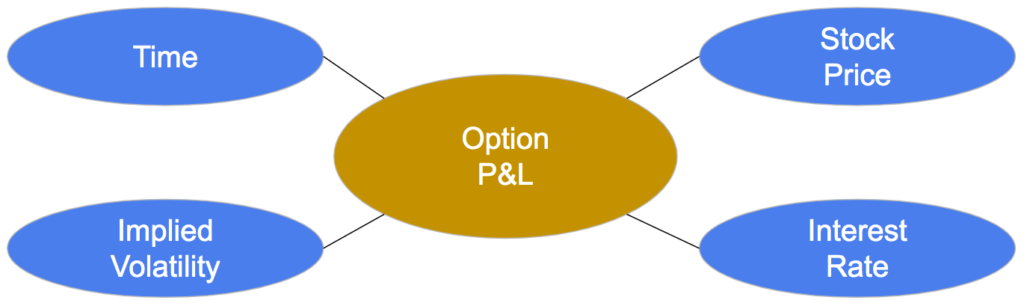
The Black-Scholes price of an option P(t, S, σ, r) is a function of time (t), the stock price (S), the implied volatility (σ) and interest rate (r).

Before the expiration of the option, its price and the P&L of the option position will vary with the dynamic of these four variables and so for risk management purposes it is key to know what is the sensitivity of the option position to changes of these different variables.

With a second order Taylor expansion of the option value over a short time interval delta t we can decompose the variation of the option price as following.

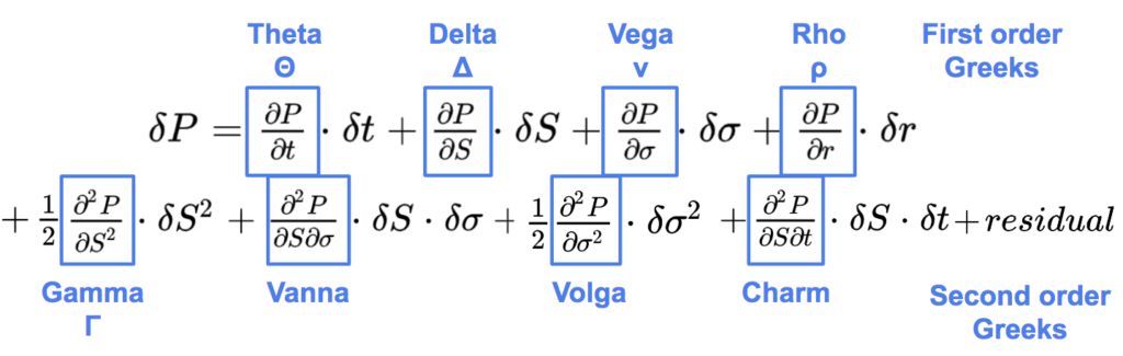
Theta, delta, vega, rho are the first order Greeks:

• The theta or time decay measures the rate at which the value of the option declines due to the passage of time.

• The delta of an option measures the change in the option’s price resulting from a change in the underlying asset. For option traders, minus delta indicates how many underlying assets are needed to be purchased or sold to hedge the directional exposure of the option position.

• Vega measures the change in the option’s price resulting from a change in the implied volatility.

• Rho measures the option’s sensitivity to changes in the risk-free rate of interest.

On the second line are the most important second order Greeks:

• The gamma measures the rate of change of the delta of an option relative to the underlying asset price. It is the second order partial derivative of the value of the option with respect to the price of the underlying asset.
• The Vanna measures the option’s sensitivity to small changes in the underlying asset price and volatility.  It is the sensitivity of the delta to changes in the volatility or the sensitivity of the vega to changes in the underlying asset price.
• The volga or vomma measures the sensitivity of the vega to a change in the implied volatility.  It is the second order partial derivative of the price of the option with respect to the implied volatility.
• The charm is the option’s sensitivity to small changes in the underlying asset price and passage of time. It is also the sensitivity of the delta to the passage of time or the sensitivity of the theta to changes in the underlying asset price.

The residual regroups other second order and higher order sensitivities.

Case Studies

We will look now at several case studies, changing market parameters and decomposing the P&L of a long out-of-the-money put option over a short time interval.

We purchase one out-of-the-money put option with a strike price K = 95, and 3 months time to maturity (T = 0.25). The underlying stock price S is equal to 100 initially.

We want to decompose the P&L of the position between t and t + δt with δt equal to one business day (δt = 1 / 252).

We assume that the interest rate and the dividend yield are both equal to zero for sake of simplicity, and we will neglect the charm P&L in the following.

The full Python code used for these analyses is available at the end of the document.

1/ Stock price down, realised volatility = market volatility, constant market volatility

First we assume that we are in Black-Scholes framework, the market implied volatility is constant, and we assume as well that the realised volatility σ_r is equal to the market one σ_I .

The realised volatility being:

the square of the change of the stock price is equal to:

We assume that the stock price is going down, so we have:

We use the following parameters:

#parameters
S0 = 100 # stock price
K = 95 # strike price
r = .0 # risk-free interest rate
q = .0 # dividend
T0 = .25 # time to maturity
sigma0 = .4 # implied volatility BS
Type = "Put"
dt = 1 / 252 # 1 business day

# Market changes between t and t + dt
dS = -S0 * sigma0 * dt**.5 # dS^2 / S^2 = sigma0^2 * dt
dsigma = .0
T1 = T0 - dt
S1 = S0 + dS
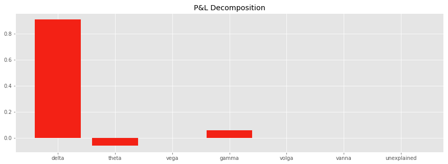
sigma1 = sigma0 + dsigma

We see on the chart below that the P&L of the option between t and t + δt is mostly explained by its directional exposure, its delta P&L. The delta P&L is positive (0.91 = -2.52 x -0.36) as the stock is going down (-2.52) and the delta of the put option is negative (-0.36).

Theta, the time decay of the option, is the cost of gamma. It is the cost for the convexity of the option measured by the gamma.

As a reminder, we have, with σ_r the realised volatility:

And if we assume that r = q = 0 we have:

So the P&L of the delta-hedged option between t and t + δt is close to:

In this first example, we assume that the realised volatility is equal to the market volatility so we have:

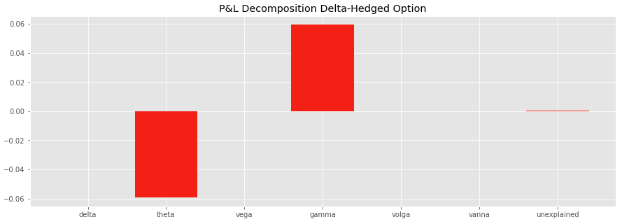
Theta P&L = – Gamma P&L (= -0.059)

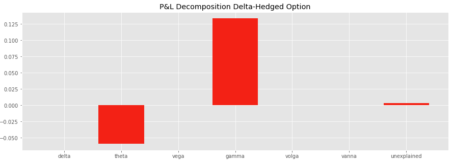
If we delta-hedge the option, by buying 0.36 stocks, the P&L of the delta-hedged option becomes very close to zero between t and t + δt, the positive contribution of the Gamma being fully offset by the negative contribution of the Theta.

2/ Stock price down, realised volatility > market volatility, constant market volatility

We assume now that the realised volatility (60%) is higher than the implied one (40%).

The stock price is still going down, with a more negative movement (-3.78 = -100 * 60% * (1/252)^ .5).

The option is still delta-hedged.

dS = -S0 * .6 * dt**.5 # realised vol = .6

The P&L of the long delta-hedged put option is positive (+0.078), Gamma P&L > Theta P&L as the realised volatility is higher than the implied volatility.

In our example, Γ = 0.019, and the P&L portion explained by the gamma and the theta is equal to

1/2 x 0.019 x 100^2 x (0.6^2 – 0.4^2) x 1 / 252 = 0.075

It is close to the P&L of the strategy between t and t + δt.

The unexplained P&L is a bit higher compared to the first case study. This is explained by a more important stock movement and a higher error of the second order Taylor expansion. Higher order sensitivities such as the “speed”, the third order partial derivative of the option with respect to the underlying asset price, are less negligible in this case.

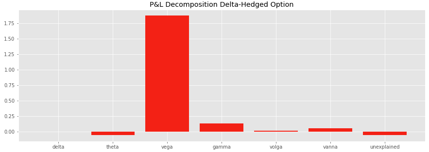
3/ Stock price down, realised volatility > market volatility, market volatility up

In this third case study, we assume as well that the market implied volatility is going up, +10%, all other assumptions being the same as in the previous case study.

dsigma = .1

As highlighted below, the change of volatility has an important impact on the P&L of the delta-hedged put option, most of it being captured by the Vega P&L.

Compared to the previous case study, the P&L of the strategy is higher (+1.95), as the long put option has a positive vega exposure, it gains when the volatility is going up.

Most of the P&L is explained by the Vega P&L (+1.87). The Vanna P&L (0.055), and to a lesser extent the Volga P&L (0.013) are positive as well.

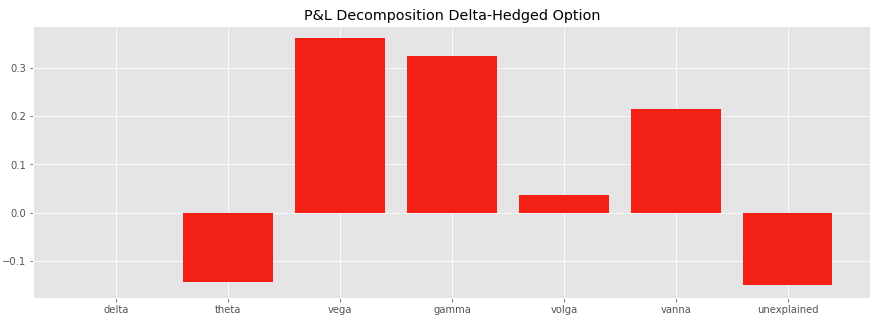
4/ Shorter time to maturity

We assume now that the option is closer to expiry, with a one week time to maturity vs three months before.

T0 = 5 / 252 # time to maturity

Market movements between t and t + δt are assumed to be the same as before, the stock is going down, with a realised volatility of 60% while the implied volatility is going up by +10%.

The delta of the option is lower. The option is closer to expiry while we assume that the moneyness of the put option is the same (95%). Now have to sell 0.174 stocks in order to delta-hedge the option.

As highlighted in the chart below, the P&L decomposition is not the same when we are very close to expiry:

• The part of the P&L explained by the vega is less important. It makes sense as the standard deviation of price returns is proportional to the square root of time, so the longer the option has until it expires, the more its price will be affected by volatility.
• The Theta P&L is more negative. Theta is the cost of convexity of the option, and there is more convexity around the strike price when the option is close to expiration as the option price converge to a piecewise linear payoff.
• Similarly, the Gamma P&L portion increases as we get closer to expiration. We observe as well a higher P&L explained by other second order Greeks, volga and vanna and a higher portion of the P&L unexplained, with a greater error of the second order Taylor expansion.

Save 10% on All Quant Next Courses with the Coupon Code: QuantNextBlog10

For students and graduates: We offer a 50% discount on all courses, please contact us if you are interested: contact@quant-next.com

Python Code

First we import the libraries that will be used and we create a class EuropeanOptionBS with Black-Scholes prices and Greeks with closed-form formulas.

#import libraries
import matplotlib.pyplot as plt
plt.style.use('ggplot')
import math
import numpy as np
import pandas as pd
from scipy.stats import norm
%matplotlib inline

#Black-Scholes price and Greeks
class EuropeanOptionBS:

    def __init__(self, S, K, T, r, q, sigma, Type):
        self.S = S
        self.K = K
        self.T = T
        self.r = r
        self.q = q        
        self.sigma = sigma
        self.Type = Type
        self.d1 = self.d1()
        self.d2 = self.d2()
        self.price = self.price()
        self.delta = self.delta()
        self.theta = self.theta()
        self.vega = self.vega()
        self.gamma = self.gamma()
        self.volga = self.volga()
        self.vanna = self.vanna()        
        
    def d1(self):
        d1 = (math.log(self.S / self.K) \
                   + (self.r - self.q + .5 * (self.sigma ** 2)) * self.T) \
                    / (self.sigma * self.T ** .5)       
        return d1

    def d2(self):
        d2 = self.d1 - self.sigma * self.T ** .5     
        return d2
    
    def price(self):
        if self.Type == "Call":
            price = self.S * math.exp(-self.q * self.T) * norm.cdf(self.d1) \
            - self.K * math.exp(-self.r * self.T) * norm.cdf(self.d2)
        if self.Type == "Put":
            price = self.K * math.exp(-self.r * self.T) * norm.cdf(-self.d2) \
            - self.S * math.exp(-self.q * self.T) * norm.cdf(-self.d1)            
        return price
    
    def delta(self):
        if self.Type == "Call":
            delta = math.exp(-self.q * self.T) * norm.cdf(self.d1)
        if self.Type == "Put":
            delta = -math.exp(-self.q * self.T) * norm.cdf(-self.d1)
        return delta
    
    def theta(self):
        if self.Type == "Call":
            theta1 = -math.exp(-self.q * self.T) * \
            (self.S * norm.pdf(self.d1) * self.sigma) / (2 * self.T ** .5)
            theta2 = self.q * self.S * math.exp(-self.q * self.T) * norm.cdf(self.d1)
            theta3 = -self.r * self.K * math.exp(-self.r * self.T) * norm.cdf(self.d2)
            theta = theta1 + theta2 + theta3
        if self.Type == "Put":
            theta1 = -math.exp(-self.q * self.T) * \
            (self.S * norm.pdf(self.d1) * self.sigma) / (2 * self.T ** .5)
            theta2 = -self.q * self.S * math.exp(-self.q * self.T) * norm.cdf(-self.d1)
            theta3 = self.r * self.K * math.exp(-self.r * self.T) * norm.cdf(-self.d2)
            theta =  theta1 + theta2 + theta3
        return theta
    
    def vega(self):
        vega = self.S * math.exp(-self.q * self.T) * self.T** .5 * norm.pdf(self.d1)
        return vega
    
    def gamma(self):
        gamma = math.exp(-self.q * self.T) * norm.pdf(self.d1) / (self.S * self.sigma * self.T** .5)
        return gamma
    
    def volga(self):
        volga = self.vega / self.sigma * self.d1 * self.d2
        return volga
    
    def vanna(self):
        vanna = -self.vega / (self.S * self.sigma * self.T** .5) * self.d2
        return vanna

Then we enter the parameters, we give one example of set of parameters here.

#parameters
S0 = 100 # stock price
K = 95 # strike price
r = .0 # risk-free interest rate
q = .0 # dividend
T0 = .25 # time to maturity
sigma0 = .4 # implied volatility BS
Type = "Put"
dt = 1 / 252 # 1 business day

# Market changes between t and t + dt
dS = -S0 * .6 * dt**.5 # realised vol = .6
dsigma = .1
T1 = T0 - dt
S1 = S0 + dS
sigma1 = sigma0 + dsigma

We calculate the P&L between t and t + δt

P0 = EuropeanOptionBS(S0, K, T0, r, q, sigma0, Type).price
P1 = EuropeanOptionBS(S1, K, T1, r, q, sigma1, Type).price
delta0 = EuropeanOptionBS(S0, K, T0, r, q, sigma0, Type).delta
isDeltaHedged = 1 #1 if is delta-hedged, 0 otherwise
dPandL = P1 - P0 - delta0 * dS * isDeltaHedged
print("P&L: " + str(dPandL))

We decompose the P&L between the contribution of the different Greeks and we plot it with a barchart.

#initial greeks
theta0 = EuropeanOptionBS(S0, K, T0, r, q, sigma0, Type).theta
vega0 = EuropeanOptionBS(S0, K, T0, r, q, sigma0, Type).vega
gamma0 = EuropeanOptionBS(S0, K, T0, r, q, sigma0, Type).gamma
volga0 = EuropeanOptionBS(S0, K, T0, r, q, sigma0, Type).volga
vanna0 = EuropeanOptionBS(S0, K, T0, r, q, sigma0, Type).vanna

#P&L attribution
delta_PandL = delta0 * dS * (1 - isDeltaHedged)
theta_PandL = theta0 * dt
vega_PandL = vega0 * dsigma
gamma_PandL = 1 / 2 * gamma0 * dS**2
volga_PandL = 1 / 2 * volga0 * dsigma**2
vanna_PandL = vanna0 * dS * dsigma
unexplained = dPandL - sum([delta_PandL, theta_PandL, vega_PandL, gamma_PandL, volga_PandL, vanna_PandL])

y = [delta_PandL, theta_PandL, vega_PandL, gamma_PandL, volga_PandL, vanna_PandL, unexplained]
x = ["delta", "theta", "vega", "gamma", "volga", "vanna","unexplained"]

fig = plt.figure(figsize=(15, 5))
plt.bar(x, y)
plt.title("P&L Decomposition")
plt.show();