Introduction to Stochastic Calculus

Foundations of Stochastic Calculus

Stochastic Calculus is a branch of mathematics that deals with random processes. Beyond probabilities it also has links with differential equations, and is widely used in finance particularly for option modelling.

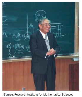
Kiyosi Itô (1915-2008) pioneered the field inventing the concept of stochastic integral and stochastic differential equations.

Itô Stochastic Integral

In order to define a stochastic integral, we first define it for elementary stochastic processes, which can be expressed as a sum of stochastic variables (A_i)_i=1..n times the indicator functions on time intervals [t_i-1,t_i): 1_[ti-1,ti)(t)=1 if t∈[t_i-1,t_i).

A stochastic process is elementary if it can be approximated by a step function:

For such process the stochastic integral between 0 and T is defines as following, with the Brownian motion W_t:

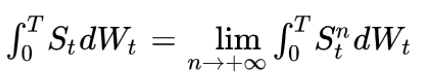
For a general process S_t the stochastic integral is defined as the limit of the integral for an elementary process converging to S_t:

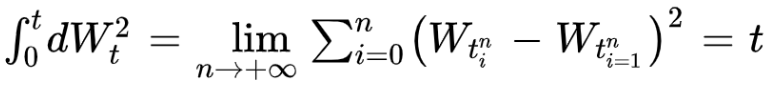
If we calculate the stochastic integrale between 0 and t of the square of dW_t we find the quadratic variation of the brownian motion. It is equal to t:

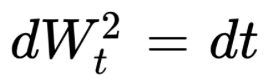
So by taking the differential we can write the following expression, very useful in stochastic differential equations and stochastic integrals:

Itô Isometry

The Ito Isometry allows to calculate the variance and the covariance of random variables which are defined by an Ito integral.

The expectation of the product of two integrals over a Brownian motion W_t is equal to the expectation of the integral of the product by replacing the square of dW_t by dt.

We have as well:

Itô Process

An Itô process X_t has the following form:

Or by taking the differential:

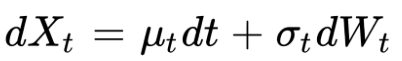
µ_t and σ_t are random processes, W_t is a Brownian motion.

Itô Lemma

Itô Lemma is one of the main result in stochastic calculus.

The derivative of a function f twice differentiable in x and differentiable in t is equal to:

X_t being an Itô process.

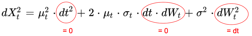
In order to demonstrate it, we do a Taylor development of f at the second order, dX² being equal to σ².dt:

Itô’s Multiplication Table

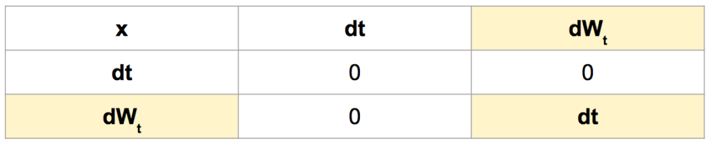
The following multiplication table is a good summary of Ito’s lemma and useful when resolving stochastic differential equations or stochastic integrals.

Stochastic Differential Equations

A stochastic differential equation (SDE) has the following form:

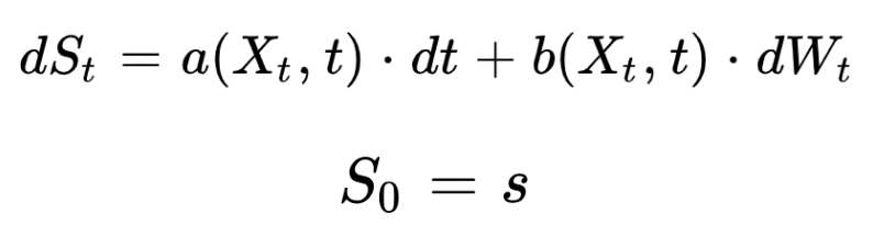
This is a generalisation of standard differential equations, where one or more terms is a stochastic process.

We only consider continuous processes, we do not consider processes with jumps here.

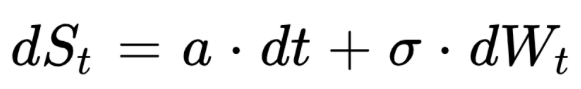
Example 1: a, σ constant

A first simple example of SDE is with a and σ constant:

By integrating between 0 and T we get the following expression for S_T.

S_T follows a gaussian distribution with a mean equal to S₀ + a.T and a variance equal to σ².T

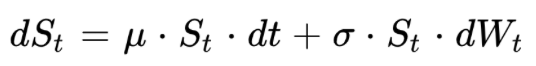
Example 2: Geometric Brownian Motion

Another important example in finance is the geometric brownian motion, often used to model the dynamic of stock prices.

This is typically the case in the famous Black-Scholes model.

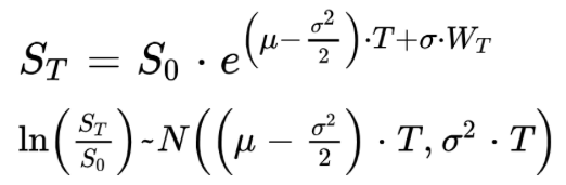
The solution of this SDE has the following expression, S_T follows a log-normal distribution:

To demonstrate it, we apply the Ito’s lemma to the fonction logarithm ln.

The first derivatives is dln(x) / dx = 1 / x while the second derivatives is d²ln(x) / dx² = – 1 / x²:

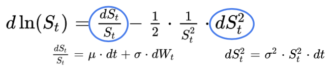
After regrouping the terms in dt and the terms in dW_t we get the following expression for the differential of ln(S_t), and we integrate it between 0 and T to finish the demonstration.

Watch the Video

Save 10% on All Quant Next Courses with the Coupon Code: QuantNextBlog10

For students and graduates: We offer a 50% discount on all courses, please contact us if you are interested: contact@quant-next.com