Implied Volatility Calculation with Newton-Raphson Algorithm

In this article, we will present the Newton-Raphson method for calculating the implied volatility from option prices.

Black-Scholes Price vs Volatility

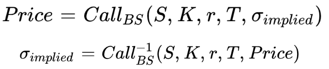
In Black-Scholes model, the price of an option is a function of five variables:

• the current price of the underlying asset,
• the strike price,
• the risk-free interest rate,
• the time to maturity and
• the volatility of the underlying asset.

The chart below shows the price of a European call option when changing the volatility, all other parameters being fixed. The option price is strictly increasing with volatility.

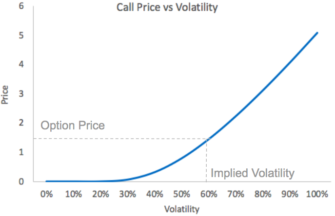
Call Price vs volatility with S = 100, K = 120, T = 1/12, r = 2%

The volatility is not directly observable, but if we know the price of the option we can determine the implied volatility.

How to Calculate the Volatility Implied by Option Prices?

There is no formula, no closed form solution for the implied volatility of an option, so we need to apply a numerical method to estimate the implied volatility from option prices.

The objective is to find the volatility level so that the Black-Scholes price is equal to the observed option price.

So we want to find the root of the function Black-Scholes price minus observed price.

Newton-Raphson Method

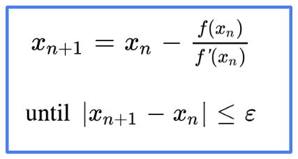
The Algorithm

The Newton Raphson method is a simple algorithm to find the root of a function: 

x₀ is our initial guess. 

Then we approximate the function by its tangent line, and our new estimate is the x-intercept of this tangent line.

We do the same with this second guess, the third guess, and so on.

We fix a tolerance level and we iterate the algorithm until the difference between two consecutive estimations is below this level.

Newton-Raphson Algorithm

Derivation

The method is derived from a simple second order Taylor expansion of the function f around x_n, ε_n is between x and x_n.

With             

 

and                    

we get the relationship between the root of the function and x_n:

When neglecting the last term, we find our new estimation of the root from our previous guess.

The convergence is quadratic, so it is quite fast.

Python Code for a Generic Newton-Raphson Algorithm

Here is a Python code with a generic Newton-Raphson algorithm.

The function has two arguments, the function f and the initial guess x0.

We approximate the derivative with finite difference.

#Import libraries
import math
import numpy as np
from scipy.stats import norm

def newton_step(f, x0):
    def df(x):
        dx = 0.00001
        return (f(x + dx) - f(x)) / dx
    return x0 - f(x0)/df(x0)

def newton(f,x0,tol):
    while (abs(newton_step(f, x0) - x0) > tol):
        x0 = newton_step(f, x0)
    return x0

We will use the Newton-Raphson algorithm to find the implied volatility of a European call option. The price of the European call price is determined by the Black-Scholes formula.

def CallPrice(S, sigma, K, T, r):
    d1 = (math.log(S / K) + (r + .5 * sigma**2) * T) / (sigma * T**.5)
    d2 = d1 - sigma * T**0.5
    n1 = norm.cdf(d1)
    n2 = norm.cdf(d2)
    DF = math.exp(-r * T)
    price=S * n1 - K * DF * n2
    return price

We want to find the root of the function Black-Scholes call price minus the target price, the only argument being the implied volatility, other parameters being fixed.

#CallPrice(vol) - TargetPrice
CallPriceVol = lambda vol: CallPrice(S, vol, K, T, r) - C

We assume that the asset price is equal to 100, the strike price is equal to 105, the maturity of the option is in six months, the risk-free interest rate is equal to 2%.

The true value of the implied volatility is 20%.

#parameters
S = 100 #asset price
K = 105 #strike price
T = .5 #time to maturity
r = .02 #risk-free interest rate
vol = .2 #implied volatility
C = CallPrice(S, vol, K, T, r) #target price

We estimate the implied volatility with the Newton-Raphson algorithm, the tolerance is fixed at 10^-8. The initial guess is arbitrarily fixed at 10%.

init = .1
tol = 10**-8
print(newton(CallPriceVol, init, tol))

In our example, the convergence is very fast, only three iterations are needed to reach the convergence with a tolerance level qt 10^-8.

x0 = init
for i in range(0, 4):
    print(x0)
    x0 = newton_step(CallPriceVol, x0)

Drawbacks

There are however several drawbacks with this method:

• The convergence is not guaranteed.
• There can be problems when the derivatives is close to zero and the convergence can be slow near local maxima/minima or in case of multiple roots.

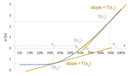
When a function is concave or convex, there is no problem of convergence of the algorithm but this is not the case with the Black-Scholes option price.

Implied Volatility Calculation in Practice

The Black-Scholes option price is an increasing function of volatility, with an upper and a lower limit.

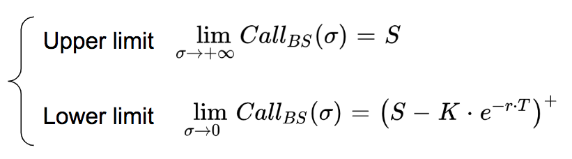
Here is an illustration of the price of the option as a function of volatility.

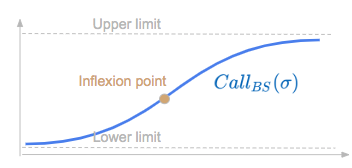
We see that there is an inflection point.

It can be shown that the function is convex on the left of the inflexion point [0,I] and concave on the right [I,+∞[ with I the inflexion point having the following expression.

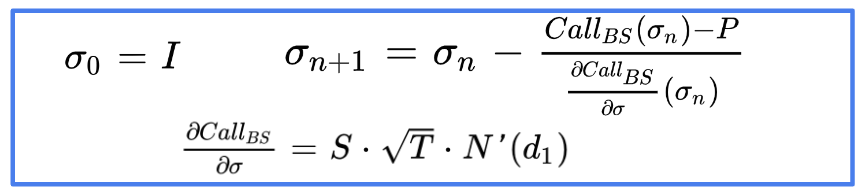
Using the inflexion point as initial guess, we can find the volatility implied by option price with the Newton-Raphson algorithm, the series of consecutive estimations (σ_n) is monotonous.

We use the vega of the call option to calculate the derivative of its price with respect to the volatility.

Source: Peter Tankov. Calibration de modèles et couverture de produits dérivés. DEA. Calibration de modèles et couverture de produits dérivés, Master “Modélisation Aléatoire”, Université Paris-Diderot (Paris 7), 2006, pp.143. ⟨cel-00664993⟩

Below is an illustration of this.

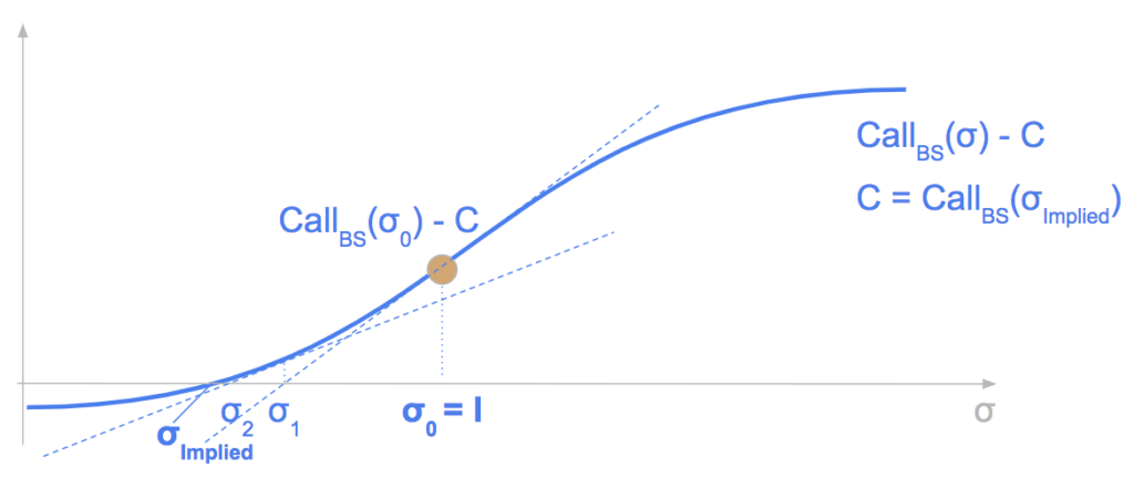
We start with the inflexion point as initial guess. Our next guess is the x-intercept of the tangent. And we continue.

σ -> Call_BS(σ) – Call_BS(σ_Implied) is convex on the left of the inflexion point.

The series is monotonous, we have σ₀ > σ₁ > … > σ_Implied.

Python Code

Below is the Python code of this algorithm.

Using above parameters for S, K, T and r we find that the inflexion point is equal to 39.39%.

def InflexionPoint(S, K, T, r):
    m = S / (K * math.exp(-r * T))
    return math.sqrt(2 * np.abs(math.log(m)) / T)

I = InflexionPoint(S, K, T, r)
print("Inflexion Point:",I)

The Newton Raphson algorithm to calculate the implied volatility is no more generic.

The derivative of the function is the Greek vega, which measures the option’s sensitivity to implied volatility and is obtained with a closed form expression.

def vega(S, sigma, K, T, r):
    d1 = (math.log(S / K) + (r + .5 * sigma**2) * T) / (sigma * T**.5)
    vega = S * T**0.5 * norm.pdf(d1)
    return vega

def ImpliedVolCall(C, S, K, r, T,tol):
    x0 = InflexionPoint(S, K, T, r)
    p = CallPrice(S, x0, K, T, r)
    v = vega(S, x0, K, T, r)
    while (abs((p - C) / v) > tol):
        x0 = x0 - (p - C) / v
        p = CallPrice(S, x0, K, T, r)
        v = vega(S, x0, K, T, r)
    return x0

tol= 10**-8
ImpliedVolCall(C, S, K, r, T,tol)

Save 10% on All Quant Next Courses with the Coupon Code: QuantNextBlog10

For students and graduates: We offer a 50% discount on all courses, please contact us if you are interested: contact@quant-next.com