From Black-Scholes to Heat Equation

The Black-Scholes Model

The Black-Scholes model is a pricing model used to determine the theoretical price of options contracts. It was developed by Fischer Black and Myron Scholes in 1973 and later refined by Robert Merton.

The model assumes that the financial market has two assets, one risky asset such as a stock price and one risk-free asset such as a bank account.

The risky asset S follows a Geometric Brownian motion, with the following stochastic differential equation:

W_t is a Wiener process, μ is the drift and σ the volatility of the stock price.

The initial model also assumed that:

• Stocks are not paying any dividend;

• We can trade continuously, with no transaction costs;

• There is no limit on short selling, no borrowing constraints;

• The risk free interest rate is constant;

• And there is no opportunities for arbitrage in the market.

Under these assumptions, Black and Scholes showed that the price of a European option on the underlying asset S with the final payoff g(S) is a solution of Black Scholes partial differential equation (PDE):

You will find the demonstration in this article: The Black-Scholes Model.

The Heat Equation

The heat equation describes how heat diffuses through a given region over time.

The heat equation is a fundamental partial differential equation that describes how heat diffuses through a given region over time. It was introduced by Joseph Fourier in 1807.

In one spatial dimension, it can be expressed as:

Where T(x, t) is the temperature at position x and time t, and α is the thermal diffusivity of the material which quantifies the rate of heat transfer from warm environment to cold environment.

Similarities between Black-Scholes and Heat Equations

Both the Black-Scholes and the heat equations are diffusion equations, of the option price for the former one, of temperature for the latter one.

Both equations have in common to have a relationship between the first order derivative with respect to time and up to a second order derivative with respect to space, if we consider S as the spatial equivalent.

The transfer of heat from warm environnement to cold environment is in a way equivalent to the erosion of option price due to the passage of time, or time decay.

If we assume that the interest rate r is equal to zero we obtain the following relationship between the first order derivative with respect to time and the second order derivative of the option price with respect to the asset price from the Black-Scholes equation.

The time decay (the theta) on the left side is related to the convexity of the option, which is controlled by the second order derivative of the option price with respect to the asset price (the gamma), and uncertainty with the volatility of the asset price.

This relationship is very similar to the heat equation.

From Black-Scholes to Heat Equation

Actually, with some changes of variables, we can transform the Black Scholes PDE into a standard heat equation.

With

,

We have

and

So we get

with the terminal condition

Solving the Black-Scholes PDE

The solution of the heat equation is given by the following integral:

It is not always possible to simplify the integral, it depends on the expression of g.

For call options

and we obtain the Black-Scholes formula by integration:

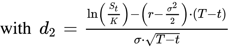
Similarly for put options

Save 10% on All Quant Next Courses with the Coupon Code: QuantNextBlog10

For students and graduates: We offer a 50% discount on all courses, please contact us if you are interested: contact@quant-next.com