Fourier Transform and Applications for Option Pricing

The Fourier Transform

The spectral decomposition of a period function via Fourier series can be generalised to any integrale function via the Fourier transform.

And we can recover the initial function from its frequency domain representation by applying the Fourier inversion theorem.

Why is it Useful for the Pricing of Options?

The characteristic function of a stochastic variable is the Fourier transform of its density function.

While it is often difficult to find the distribution function for a few stochastic processes, it is more simple to get their characteristic function, as it can be derived as the solution of a partial differential equation using the Feynman Kac theorem (see for example Cornelis W Oosterlee, Lech A Grzelak (2020): “Mathematical Modeling And Computation In Finance” ).

And if we know the characteristic function we can recover the density function by applying the Fourier inversion theorem.

And we can easily derive the price of a call option using the characteristic function instead of the density function of the log of the asset price with a semi-analytic solution (see for example Ricardo Crisóstomo (2014), “An Analysis of the Heston Stochastic Volatility Model: Implementation and Calibration using Matlab”).

The price of the call option has a similar expression as in the Black-Scholes formula, instead of using the density function, the probabilities are calculated with an integral via the characteristic function.

This is typically the case for the Heston model (see Heston, Steven L. (1993), “A closed-form  solution for options with stochastic volatility with applications to bond and currency options”).

In the Heston model, under the risk neutral probability, the dynamic of the asset price and its variance can be expressed as:

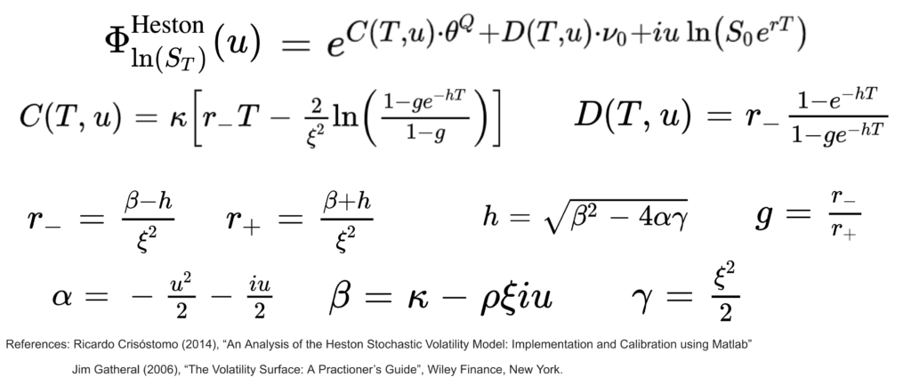
Here is the expression of the characteristic function of the log price under the Heston model:

The computation of the Discrete Fourier Transform (DFT) can be time consuming with O(N²) complexity. The Fast Fourier Transform (FFT) are efficient algorithms for reducing the complexity from O(N²) to (O(N.log(N)). They work by dividing the DFT problem into smaller sub-problems (divide-and-conquer) and recursively computing them, with a significant reduction in the number of arithmetic operations (reference: https://en.wikipedia.org/wiki/Fast_Fourier_transform).

Save 10% on All Quant Next Courses with the Coupon Code: QuantNextBlog10

For students and graduates: We offer a 50% discount on all courses, please contact us if you are interested: contact@quant-next.com