Artificial Neural Network for Option Pricing with Python Code

The valuation and the risk management of options can be quickly complex. It depends on the option’s feature and the pricing model. There is often no closed-form solution for the pricing of the derivatives and it involves multiple dimensions.

There is a vaste litterature on numerical methods such as binomial / trinomial tree, finite difference, or Monte-Carlo methods to price options, but they can be very time consuming in some cases.

In this article we analyse an alternative method using artificial neural network (ANN) to price options looking at the efficiency of the ANN to learn the Black-Scholes option pricing formulas.

Artificial Neural Network

An artificial neural network (ANN) is a computational system inspired by the biological neural network found in animal brains. It consists of a collection of interconnected nodes, called neurons, which are organised into layers.

The neurons in each layer receive weighted inputs, process them through an activation function, and then pass the results to the neurons in the next layer. The neurons in the input layer receive input signals from the external environment while the neurons in the output layer produce the output. Hidden layers are intermediate layers between input and output layers.

The connections between neurons are weighted, which means that some inputs have a stronger influence on the output of the neuron than others. These weights are adjusted during training to improve the performance of the network for a specific objective.

Below is an example of a multiple layer perceptron with three neurons in the input layer, two hidden layers, each of them having four neurons, and one neuron in the output layer.

Example of Multiple Layer Perceptron

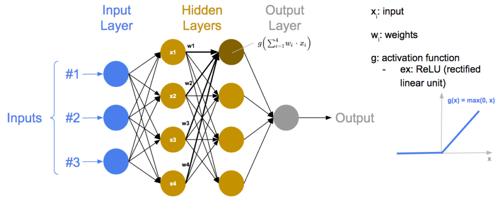
The rectified linear activation function or ReLU is a piecewise linear function that will output the input if it is positive and zero otherwise. It is widely used as the default activation function in neural networks due to its ability to facilitate easier training and often yielding good performance.

ANN is an example of supervised learning algorithm, it can be used for both classification or regression. 

Here we want to use an ANN to approximate a function.

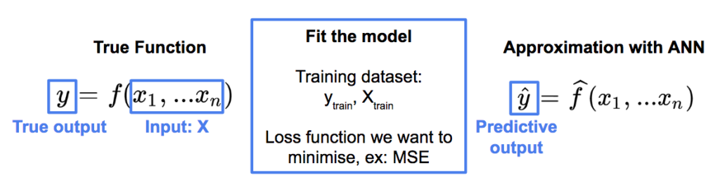
We know the true function f, which will return the true output y from inputs X. We want to approximate it with the ANN.

From the input X, it will return a predictive output that we can compare to the true value.

In order to fit the model, we will define a training dataset where the model will learn, using a loss function in order to measure the difference between the estimation from the model and the true value, we want to minimise it. The mean squared error MSE is an example of loss function.

We use here the Adam algorithm (Adaptive Moment Estimation) to minimise the loss function. It is a popular optimization algorithm used in deep learning and particularly for training neural networks. It is an extension of the stochastic gradient descent optimization algorithm.

Two important inputs in the algorithm are the epoch and the batch size, they are both related to how the model learns from the data and they have to be chosen carefully.

The Batch size is the number of training examples used in one iteration of the optimization algorithm. If the batch size is set to 16 as in our example, the model will take 16 data points at a time and update the weights of the model based on the average loss of those 16 samples. A larger batch size leads to a more stable training process but requires more memory to process. They are in general chosen to be a power of 2 as CPU and GPU memory architectures are organized in powers of 2, and it can be faster and more efficient to do so.

An epoch corresponds to the number of times the algorithm sees the entire training dataset. For example, if we have 750 data points in our training data set and a batch size of 16, then one epoch would involve 47 iterations (750 / 16 = 46.875).  Training more epochs can improve the accuracy of the model but it can also lead to overfitting, so it is important to find a good balance.

A First Simple Example: Estimation of a Parabolic Function

Let’s have a look at a first simple example with Python code. We will train a neural network to estimate a parabolic function. We will build the ANN with Keras framework in Python. First we import the libraries that will be used.

#import libraries
import matplotlib.pyplot as plt
plt.style.use('ggplot')
import math
import numpy as np
import pandas as pd
from scipy.stats import norm
from sklearn.model_selection import train_test_split
from keras.models import Sequential
from keras.layers import Dense
from sklearn.metrics import r2_score

Here is the function we want to estimate:

#function we want to approximate 
#y = 3 * x^2 + 6
def f(x):
    return 3 * x**2 + 6
x = np.arange(-10, 10.01, .01)
y = f(x)

We plot it.

plt.figure(figsize = (10,5))
plt.plot(x, y)
plt.xlabel("x")
plt.ylabel("y")
plt.show()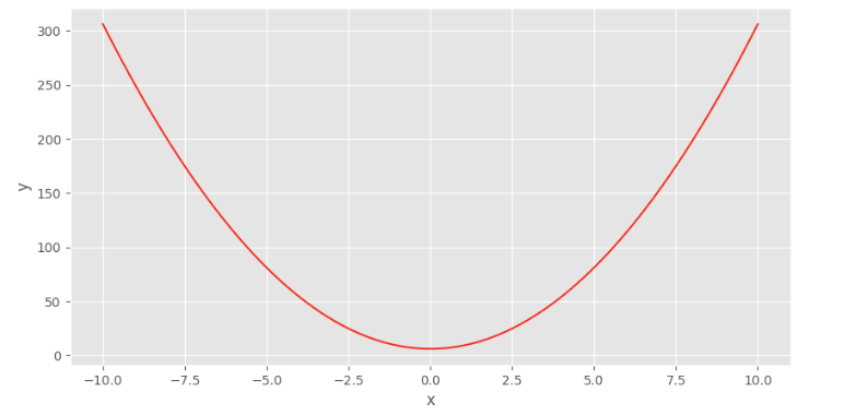

We use values between -10 and 10 for x in the dataset. We split the dataset between the training and test dataset, with a split of 75% for the training and 25% for the test.

#build the training and test datasets
X = x
y = y
X_train, X_test, y_train, y_test = \
train_test_split(X, y, test_size=0.25, random_state=0)

Then we build the ANN with four layers, with 10 neurons each.

ANN = Sequential()
ANN.add(Dense(10,input_dim = 1, activation = 'relu'))
ANN.add(Dense(10, activation = 'relu'))
ANN.add(Dense(10, activation = 'relu'))
ANN.add(Dense(10, activation = 'relu'))         
ANN.add(Dense(1))

We use the mean squared error for the loss function and the Adam algorithm to minimize it, fitting the model on the training dataset. We use a batch size equal to 16 and 150 epochs here.

#Loss function = MSE, optimizer: Adam
ANN.compile(loss = 'mean_squared_error', optimizer='adam')
# fit the ANN on the training dataset
ANN.fit(X_train, y_train, epochs = 150, batch_size = 16)

We estimate the values on the test dataset.

#prediction
y_pred = ANN.predict(X_test)

And we compare the estimations from the model with the real values, with a strong relationship between the two.

#Comparison real values and predictions on test dataset
plt.figure(figsize = (15,10))
plt.scatter(y_test, y_pred)
plt.xlabel("Real Value")
plt.ylabel("ANN Value")
plt.annotate("r-squared = {:.3f}".format(r2_score(y_test, y_pred)), (20, 1), size = 15)
plt.show();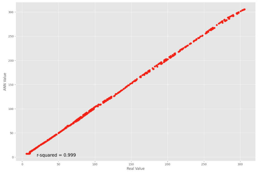

However, the efficiency of the model is more limited for extrapolating the curve.

#Extrapolation with ANN
X = np.arange(-20, 20.01, .01)
y = f(X)
y_pred = ANN.predict(X)

As highlighted on the chart on the right, when using input data out of the initial range between -10 and + 10 the model tends to underestimate the output value in this example. Other neural network or different parameters could potentially improve the model.

plt.figure(figsize = (15,10))
plt.plot(X, y, label = "Real value")
plt.plot(X, y_pred, label = "Estimation with ANN")
plt.xlabel("x")
plt.ylabel("y")
plt.legend()
plt.show()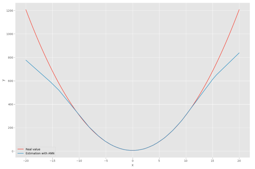

Let’s see if the ANN works well to estimate the Black-Scholes formula.

Black-Scholes Formula with ANN

We know the price of a european call option in the Black-Scholes model, it is given by the following closed form solution.

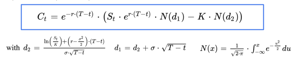
The option price is a function of five variables, the asset price S, the strike price K, the time to maturity capital T minus t, the volatility sigma and the risk free interest rate r.

As the option price is linear homogenous in S and K, it can be reduced to four variables, fixing S at 100 for example.

We define the option price of european call and put options in the Black-Scholes framework.

class EuropeanOptionBS:

    def __init__(self, S, K, T, r, q, sigma,Type):
        self.S = S
        self.K = K
        self.T = T
        self.r = r
        self.q = q        
        self.sigma = sigma
        self.Type = Type
        self.d1 = self.d1()
        self.d2 = self.d2()
        self.price = self.price()
        
    def d1(self):
        d1 = (math.log(self.S / self.K) \
                   + (self.r - self.q + .5 * (self.sigma ** 2)) * self.T) \
                    / (self.sigma * self.T ** .5)       
        return d1

    def d2(self):
        d2 = self.d1 - self.sigma * self.T ** .5     
        return d2
    
    def price(self):
        if self.Type == "Call":
            price = self.S * math.exp(-self.q * self.T) * norm.cdf(self.d1) \
            - self.K * math.exp(-self.r *self.T) * norm.cdf(self.d2)
        if self.Type == "Put":
            price = self.K * math.exp(-self.r * self.T) * norm.cdf(-self.d2) \
            - self.S * math.exp(-self.q * self.T) * norm.cdf(-self.d1)            
        return price

And we create the dataset to train the model, with a large number of values for the four variables and the corresponding european call option prices.

#dataset
r = np.arange(.0, .1, .01) #interest rates
Strike = np.arange(50, 155, 5) #strike price
T = np.arange(0.1, 2.1, 0.1) #time to maturity
sigma = np.arange(0.1, 2.1, .1) #volatility

data = []
for r_ in r:
    for Strike_ in Strike:
        for T_ in T:
            for sigma_ in sigma:
                data.append([r_, Strike_, T_, sigma_, \
                             EuropeanOptionBS(100, Strike_, T_, r_, 0, sigma_, "Call").price])
data = np.asarray(data)

Again we split the dataset between training and test.

#training and test datasets
X = data[:,:4] #params r, strike, T, sigma
y = data[:,4:5] #call price
X_train, X_test, y_train, y_test = train_test_split(X, y, test_size=0.25, random_state=0)

We create and we fit the neural network on the training dataset. We use again a neural network with four layers, 10 neurons in each, the input dimension is now 4.

#ANN with four layers, 10 neurons each
#activation function: ReLU
ANN = Sequential()
ANN.add(Dense(10,input_dim = 4, activation = 'relu'))
ANN.add(Dense(10, activation = 'relu'))
ANN.add(Dense(10, activation = 'relu'))
ANN.add(Dense(10, activation = 'relu'))         
ANN.add(Dense(1))

We did not change the number of epochs (150) or the batch size (16). Of course the training takes more time compared to the previous simple example as the training dataset is bigger, the function being more complex with four variables instead of one. 

#Loss function = MSE, optimizer: Adam
ANN.compile(loss = 'mean_squared_error', optimizer='adam')
# fit the ANN on the training dataset
ANN.fit(X_train, y_train, epochs = 150, batch_size = 16)

We still get good results when comparing estimated and real values in the test dataset.

#prediction
y_pred = ANN.predict(X_test)

#Comparison real values and predictions on test dataset
plt.figure(figsize = (15,10))
plt.scatter(y_test, y_pred)
plt.xlabel("Real Value")
plt.ylabel("ANN Value")
plt.annotate("r-squared = {:.3f}".format(r2_score(y_test, y_pred)), (20, 1), size = 15)
plt.show();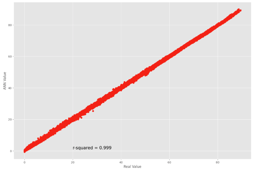

Now, we compare the price of an option with a strike price at 120, a time to maturity at 6 months (0.5), the risk-free interest rate at 5% and the implied volatility at 30% when changing the asset price.

K = 120 #strike price
r = 0.05 #risk-free interest rate
sigma = .3 #implied volatiltiy
T = .5 #time to maturity
S = np.arange(50, 151, 1) #asset prices

PriceBS = [EuropeanOptionBS(S_, K, T, r, 0, sigma, "Call").price for S_ in S]
PriceANN = [S_ / 100 * \
            ANN.predict(np.array([[r, K / S_ * 100, T, sigma]]))[0][0] for S_ in S]

Even if we obtain good approximations for the prices, the estimation of the greeks may be more unstable which can be an issue of course. 

#Comparison BS vs ANN prices
plt.figure(figsize = (15,10))
plt.plot(S, PriceBS, label = "Black-Scholes price")
plt.plot(S, PriceANN, label = "ANN price")
plt.xlabel("Asset Price")
plt.ylabel("Call Price")
plt.show();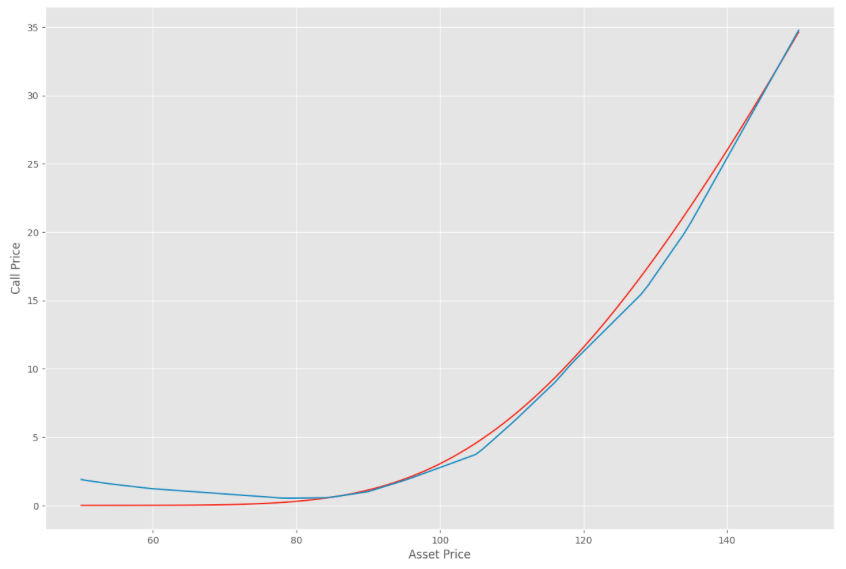

Moreover, we see on the left side of the chart that the model price of the call option increases when the asset price decreases which is a violation of the call spread arbitrage condition.

The no arbitrage conditions such as the call spread, butterfly spread or calendar spread may be violated so it may require additional regularisation techniques.

If you are interested in further reading, you will find many academic articles on the topic, this one proposes a review of the literature on neural network for option pricing and hedging: Johannes Ruf, Weiguan Wang (2020): “Neural networks for option pricing and hedging: a literature review”.

Watch the Video

Save 10% on All Quant Next Courses with the Coupon Code: QuantNextBlog10

For students and graduates: We offer a 50% discount on all courses, please contact us if you are interested: contact@quant-next.com